过关斩将打进Kaggle竞赛Top 0.3%,我是这样做的

作者 | Lavanya Shukla
译者 | Monanfei
责编 | 夕颜
出品 | AI科技大本营(id:rgznai100)
导读:刚开始接触数据竞赛时,我们可能会被一些高大上的技术吓到。各界大佬云集,各种技术令人眼花缭乱,新手们就像蜉蝣一般渺小无助。今天本文就分享一下在 kaggle 的竞赛中,参赛者取得 top0.3% 的经验和技巧。让我们开始吧!
Top 0.3% 模型概览
赛题和目标
数据集中的每一行都描述了某一匹马的特征
在已知这些特征的条件下,预测每匹马的销售价格
预测价格对数和真实价格对数的RMSE(均方根误差)作为模型的评估指标。将RMSE转化为对数尺度,能够保证廉价马匹和高价马匹的预测误差,对模型分数的影响较为一致。
模型训练过程中的重要细节
交叉验证:使用12-折交叉验证
模型:在每次交叉验证中,同时训练七个模型(ridge, svr, gradient boosting, random forest, xgboost, lightgbm regressors)
Stacking 方法:使用 xgboot 训练了元 StackingCVRegressor 学习器
模型融合:所有训练的模型都会在不同程度上过拟合,因此,为了做出最终的预测,将这些模型进行了融合,得到了鲁棒性更强的预测结果
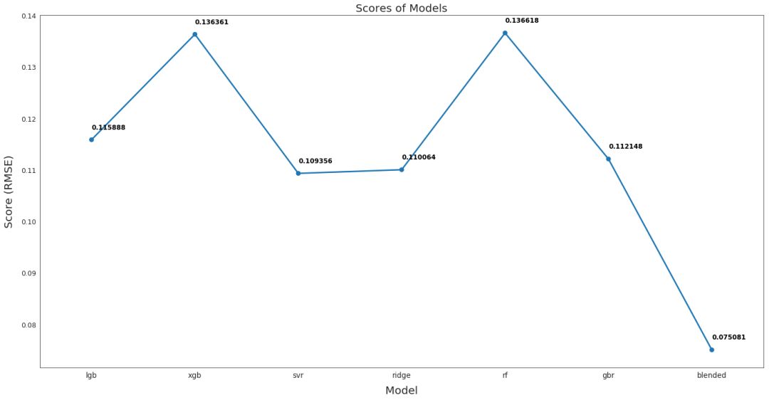
模型性能
从下图可以看出,融合后的模型性能最好,RMSE 仅为 0.075,该融合模型用于最终预测。
In[1]:
from IPython.display import Image
Image("../input/kernel-files/model_training_advanced_regression.png")
Output[1]:
现在让我们正式开始吧!
In[2]:
# Essentials
import numpy as np
import pandas as pd
import datetime
import random
# Plots
import seaborn as sns
import matplotlib.pyplot as plt # Models
from sklearn.ensemble import RandomForestRegressor, GradientBoostingRegressor, AdaBoostRegressor, BaggingRegressor
from sklearn.kernel_ridge import KernelRidge
from sklearn.linear_model import Ridge, RidgeCV
from sklearn.linear_model import ElasticNet, ElasticNetCV
from sklearn.svm import SVR
from mlxtend.regressor import StackingCVRegressor
import lightgbm as lgb
from lightgbm import LGBMRegressor
from xgboost import XGBRegressor # Stats
from scipy.stats import skew, norm
from scipy.special import boxcox1p
from scipy.stats import boxcox_normmax # Misc
from sklearn.model_selection import GridSearchCV
from sklearn.model_selection import KFold, cross_val_score
from sklearn.metrics import mean_squared_error
from sklearn.preprocessing import OneHotEncoder
from sklearn.preprocessing import LabelEncoder
from sklearn.pipeline import make_pipeline
from sklearn.preprocessing import scale
from sklearn.preprocessing import StandardScaler
from sklearn.preprocessing import RobustScaler
from sklearn.decomposition import PCA pd.set_option('display.max_columns', None) # Ignore useless warnings
import warnings
warnings.filterwarnings(action="ignore")
pd.options.display.max_seq_items = 8000
pd.options.display.max_rows = 8000 import os
print(os.listdir("../input/kernel-fi
Output[2]:
['model_training_advanced_regression.png']
In[3]:
# Read in the dataset as a dataframe
train = pd.read_csv('../input/house-prices-advanced-regression-techniques/train.csv')
test = pd.read_csv('../input/house-prices-advanced-regression-techniques/test.csv')
train.shape, test.shape
Output[3]:
((1460, 81), (1459, 80))
EDA
目标
数据集中的每一行都描述了某一匹马的特征
在已知这些特征的条件下,预测每匹马的销售价格
对原始数据进行可视化
In[4]:
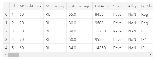
# Preview the data we're working with
train.head()
Output[5]:
SalePrice:目标值的特性探究
In[5]:
sns.set_style("white")
sns.set_color_codes(palette='deep')
f, ax = plt.subplots(figsize=(8, 7))
#Check the new distribution
sns.distplot(train['SalePrice'], color="b");
ax.xaxis.grid(False)
ax.set(ylabel="Frequency")
ax.set(xlabel="SalePrice")
ax.set(title="SalePrice distribution")
sns.despine(trim=True, left=True)
plt.show() 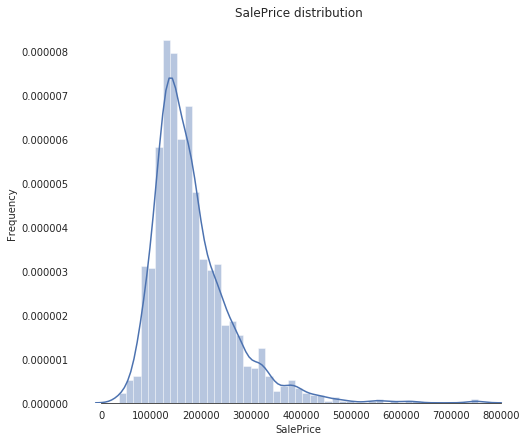
In[6]:
# Skew and kurt
print("Skewness: %f" % train['SalePrice'].skew())
print("Kurtosis: %f" % train['SalePrice'].kurt())
Skewness: 1.882876
Kurtosis: 6.536282
可用的特征:深入探索
数据可视化
In[7]:
# Finding numeric features
numeric_dtypes = ['int16', 'int32', 'int64', 'float16', 'float32', 'float64']
numeric = []
for i in train.columns: if train[i].dtype in numeric_dtypes: if i in ['TotalSF', 'Total_Bathrooms','Total_porch_sf','haspool','hasgarage','hasbsmt','hasfireplace']: pass else: numeric.append(i)
# visualising some more outliers in the data values
fig, axs = plt.subplots(ncols=2, nrows=0, figsize=(12, 120))
plt.subplots_adjust(right=2)
plt.subplots_adjust(top=2)
sns.color_palette("husl", 8)
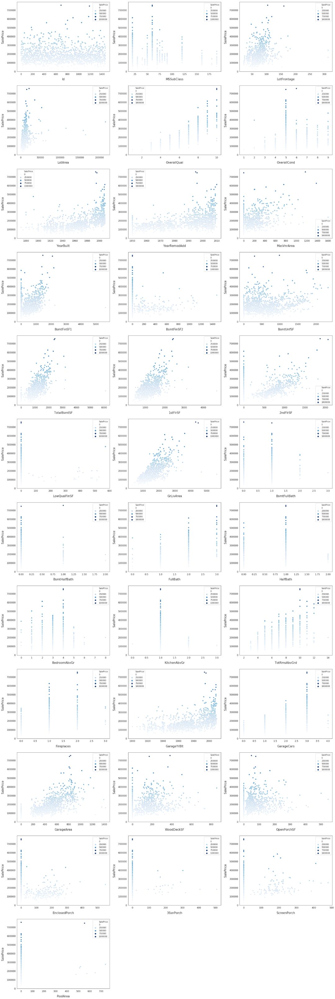
for i, feature in enumerate(list(train[numeric]), 1): if(feature=='MiscVal'): break plt.subplot(len(list(numeric)), 3, i) sns.scatterplot(x=feature, y='SalePrice', hue='SalePrice', palette='Blues', data=train) plt.xlabel('{}'.format(feature), size=15,labelpad=12.5) plt.ylabel('SalePrice', size=15, labelpad=12.5) for j in range(2): plt.tick_params(axis='x', labelsize=12) plt.tick_params(axis='y', labelsize=12) plt.legend(loc='best', prop={'size': 10}) plt.show()
探索这些特征以及 SalePrice 的相关性
In[8]:
corr = train.corr()
plt.subplots(figsize=(15,12))
sns.heatmap(corr, vmax=0.9, cmap="Blues", square=True)
Output[8]:
<matplotlib.axes._subplots.AxesSubplot at 0x7ff0e416e4e0>
选取部分特征,可视化它们和 SalePrice 的相关性
Input[9]:
data = pd.concat([train['SalePrice'], train['OverallQual']], axis=1)
f, ax = plt.subplots(figsize=(8, 6))
fig = sns.boxplot(x=train['OverallQual'], y="SalePrice", data=data)
fig.axis(ymin=0, ymax=800000); 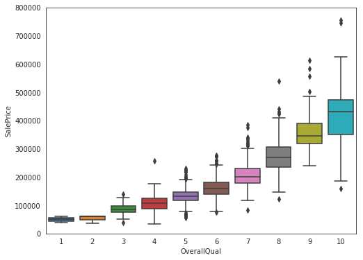
Input[10]:
data = pd.concat([train['SalePrice'], train['YearBuilt']], axis=1)
f, ax = plt.subplots(figsize=(16, 8))
fig = sns.boxplot(x=train['YearBuilt'], y="SalePrice", data=data)
fig.axis(ymin=0, ymax=800000);
plt.xticks(rotation=45); 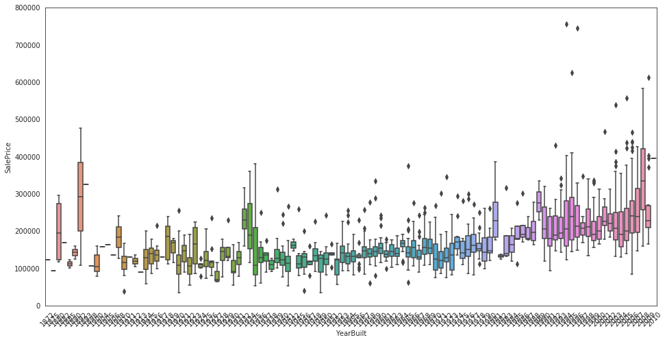
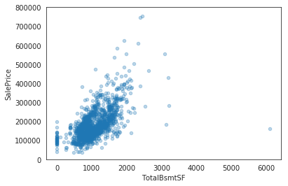
Input[11]:
data = pd.concat([train['SalePrice'], train['TotalBsmtSF']], axis=1)
data.plot.scatter(x='TotalBsmtSF', y='SalePrice', alpha=0
.3, ylim=(0,800000));
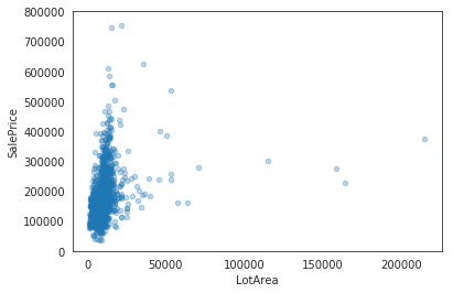
Input[12]:
data = pd.concat([train['SalePrice'], train['LotArea']], axis=1)
data.plot.scatter(x='LotArea', y='SalePrice', alpha=0.3, y
lim=(0,800000));
Input[13]:
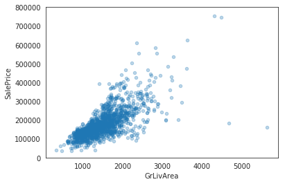
data = pd.concat([train['SalePrice'], train['GrLivArea']], axis=1)
data.plot.scatter(x='GrLivArea', y='SalePrice', alpha=0.3,
ylim=(0,800000));
Input[14]:
# Remove the Ids from train and test, as they are unique for each row and hence not useful for the model
train_ID = train['Id']
test_ID = test['Id']
train.drop(['Id'], axis=1, inplace=True)
test.drop(['Id'], axis=1, inplace=True)
train.shape, test.shape
Output[14]:
((1460, 80), (1459, 79))
可视化 salePrice 的分布
Input[15]:
sns.set_style("white")
sns.set_color_codes(palette='deep')
f, ax = plt.subplots(figsize=(8, 7))
#Check the new distribution
sns.distplot(train['SalePrice'], color="b");
ax.xaxis.grid(False)
ax.set(ylabel="Frequency")
ax.set(xlabel="SalePrice")
ax.set(title="SalePrice distribution")
sns.despine(trim=True, left=True)
plt.show()
从上图中可以看出,SalePrice 有点向右边倾斜,由于大多数机器学习模型对非正态分布的数据的效果不佳,因此,我们对数据进行变换,修正这种倾斜:log(1+x)
Input[16]:
# log(1+x) transform
train["SalePrice"] = np.log1p(train["SalePrice"])
对 SalePrice 重新进行可视化
Input[17]:
sns.set_style("white")
sns.set_color_codes(palette='deep')
f, ax = plt.subplots(figsize=(8, 7))
#Check the new distribution
sns.distplot(train['SalePrice'] , fit=norm, color="b");	# Get the fitted parameters used by the function
(mu, sigma) = norm.fit(train['SalePrice'])
print( '\n mu = {:.2f} and sigma = {:.2f}\n'.format(mu, sigma))	#Now plot the distribution
plt.legend(['Normal dist. ($\mu=$ {:.2f} and $\sigma=$ {:.2f} )'.format(mu, sigma)],	loc='best')
ax.xaxis.grid(False)
ax.set(ylabel="Frequency")
ax.set(xlabel="SalePrice")
ax.set(title="SalePrice distribution")
sns.despine(trim=True, left=True)	plt.show
mu = 12.02 and sigma = 0.40
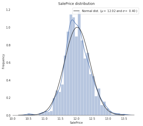
从图中可以看到,当前的 SalePrice 已经变成了正态分布
Input[18]:
# Remove outliers
train.drop(train[(train['OverallQual']<5) & (train['SalePrice']>200000)].index, inplace=True)
train.drop(train[(train['GrLivArea']>4500) & (train['SalePrice']<300000)].index, inplace=True)
train.reset_index(drop=True, inplace=True)
Input[19]:
# Split features and labels
train_labels = train['SalePrice'].reset_index(drop=True)
train_features = train.drop(['SalePrice'], axis=1)
test_features = test
# Combine train and test features in order to apply the feature transformation pipeline to the entire dataset
all_features = pd.concat([train_features, test_features]).reset_index(drop=True)
all_features.shape
Input[19]:
(2917, 79)
填充缺失值
Input[20]:
# determine the threshold for missing values
def percent_missing(df):	data = pd.DataFrame(df)	df_cols = list(pd.DataFrame(data))	dict_x = {}	for i in range(0, len(df_cols)):	dict_x.update({df_cols[i]: round(data[df_cols[i]].isnull().mean()*100,2)})	return dict_x	missing = percent_missing(all_features)
df_miss = sorted(missing.items(), key=lambda x: x[1], reverse=True)
print('Percent of missing data')
df_miss[0:10]
Percent of missing data
Output[20]:
[('PoolQC', 99.69),
('MiscFeature', 96.4),
('Alley', 93.21),
('Fence', 80.43),
('FireplaceQu', 48.68),
('LotFrontage', 16.66),
('GarageYrBlt', 5.45),
('GarageFinish', 5.45),
('GarageQual', 5.45),
('GarageCond', 5.45)]
Input[21]:
# Visualize missing values
sns.set_style("white")
f, ax = plt.subplots(figsize=(8, 7))
sns.set_color_codes(palette='deep')
missing = round(train.isnull().mean()*100,2)
missing = missing[missing > 0]
missing.sort_values(inplace=True)
missing.plot.bar(color="b")
# Tweak the visual presentation
ax.xaxis.grid(False)
ax.set(ylabel="Percent of missing values")
ax.set(xlabel="Features")
ax.set(title="Percent missing data by feature")
sns.despine(trim=True, left=True) 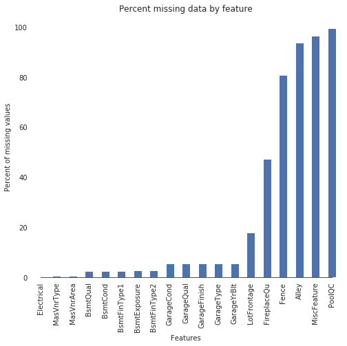
接下来,我们将分别对每一列填充缺失值
Input[22]:
# Some of the non-numeric predictors are stored as numbers; convert them into strings
all_features['MSSubClass'] = all_features['MSSubClass'].apply(str)
all_features['YrSold'] = all_features['YrSold'].astype(str)
all_features['MoSold'] = all_features['MoSold'].astype(str)
Input[23]:
def handle_missing(features): # the data description states that NA refers to typical ('Typ') values features['Functional'] = features['Functional'].fillna('Typ') # Replace the missing values in each of the columns below with their mode features['Electrical'] = features['Electrical'].fillna("SBrkr") features['KitchenQual'] = features['KitchenQual'].fillna("TA") features['Exterior1st'] = features['Exterior1st'].fillna(features['Exterior1st'].mode()[0]) features['Exterior2nd'] = features['Exterior2nd'].fillna(features['Exterior2nd'].mode()[0]) features['SaleType'] = features['SaleType'].fillna(features['SaleType'].mode()[0]) features['MSZoning'] = features.groupby('MSSubClass')['MSZoning'].transform(lambda x: x.fillna(x.mode()[0])) # the data description stats that NA refers to "No Pool" features["PoolQC"] = features["PoolQC"].fillna("None") # Replacing the missing values with 0, since no garage = no cars in garage for col in ('GarageYrBlt', 'GarageArea', 'GarageCars'): features[col] = features[col].fillna(0) # Replacing the missing values with None for col in ['GarageType', 'GarageFinish', 'GarageQual', 'GarageCond']: features[col] = features[col].fillna('None') # NaN values for these categorical basement features, means there's no basement for col in ('BsmtQual', 'BsmtCond', 'BsmtExposure', 'BsmtFinType1', 'BsmtFinType2'): features[col] = features[col].fillna('None') # Group the by neighborhoods, and fill in missing value by the median LotFrontage of the neighborhood features['LotFrontage'] = features.groupby('Neighborhood')['LotFrontage'].transform(lambda x: x.fillna(x.median())) # We have no particular intuition around how to fill in the rest of the categorical features # So we replace their missing values with None objects = [] for i in features.columns: if features[i].dtype == object: objects.append(i) features.update(features[objects].fillna('None')) # And we do the same thing for numerical features, but this time with 0s numeric_dtypes = ['int16', 'int32', 'int64', 'float16', 'float32', 'float64'] numeric = [] for i in features.columns: if features[i].dtype in numeric_dtypes: numeric.append(i) features.update(features[numeric].fillna(0)) return features all_features = handle_missing(all_featuresInput[24]:
# Let's make sure we handled all the missing values
missing = percent_missing(all_features)
df_miss = sorted(missing.items(), key=lambda x: x[1], reverse=True)
print('Percent of missing data')
df_miss[0:10]
Output[14]:
Percent of missing data
[('MSSubClass', 0.0),
('MSZoning', 0.0),
('LotFrontage', 0.0),
('LotArea', 0.0),
('Street', 0.0),
('Alley', 0.0),
('LotShape', 0.0),
('LandContour', 0.0),
('Utilities', 0.0),
('LotConfig', 0.0)]
从上面的结果可以看到,所有缺失值已经填充完毕
调整分布倾斜的特征
Input[25]:
# Fetch all numeric features
numeric_dtypes = ['int16', 'int32', 'int64', 'float16', 'float32', 'float64']
numeric = []
for i in all_features.columns:	if all_features[i].dtype in numeric_dtypes:	numeric.append(i)
Input[26]:
# Create box plots for all numeric features
sns.set_style("white")
f, ax = plt.subplots(figsize=(8, 7))
ax.set_xscale("log")
ax = sns.boxplot(data=all_features[numeric] , orient="h", palette="Set1")
ax.xaxis.grid(False)
ax.set(ylabel="Feature names")
ax.set(xlabel="Numeric values")
ax.set(title="Numeric Distribution of Features")
sns.despine(trim=True, left=True) 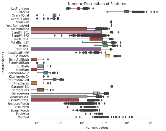
Input[27]:
# Find skewed numerical features
skew_features = all_features[numeric].apply(lambda x: skew(x)).sort_values(ascending=False)	high_skew = skew_features[skew_features > 0.5]
skew_index = high_skew.index	print("There are {} numerical features with Skew > 0.5 :".format(high_skew.shape[0]))
skewness = pd.DataFrame({'Skew' :high_skew})
skew_features.head(10
Output[27]:
There are 25 numerical features with Skew > 0.5 :
MiscVal 21.939672
PoolArea 17.688664
LotArea 13.109495
LowQualFinSF 12.084539
3SsnPorch 11.372080
KitchenAbvGr 4.300550
BsmtFinSF2 4.144503
EnclosedPorch 4.002344
ScreenPorch 3.945101
BsmtHalfBath 3.929996
dtype: float64
使用 scipy 的函数 boxcox1来进行 Box-Cox 转换,将数据正态化
Input[28]:
# Normalize skewed features
for i in skew_index:	all_features[i] = boxcox1p(all_features[i], 	boxcox_normmax(all_features[i] + 1))
Input[29]:
# Let's make sure we handled all the skewed values
sns.set_style("white")
f, ax = plt.subplots(figsize=(8, 7))
ax.set_xscale("log")
ax = sns.boxplot(data=all_features[skew_index] , orient="h", palette="Set1")
ax.xaxis.grid(False)
ax.set(ylabel="Feature names")
ax.set(xlabel="Numeric values")
ax.set(title="Numeric Distribution of Features")
sns.despine(trim=True, left=True) 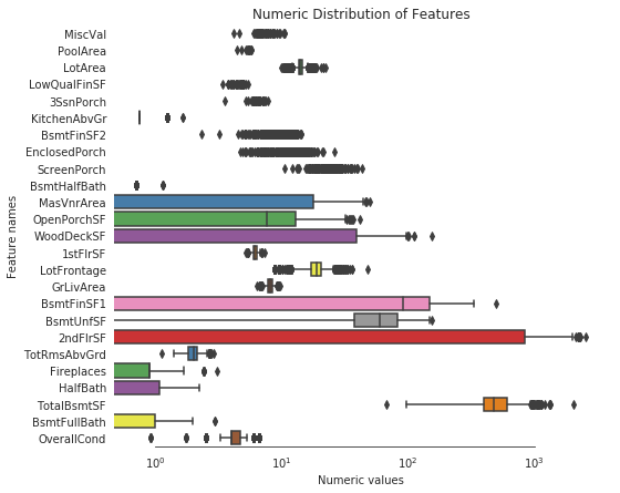
从上图可以看到,所有特征都看上去呈正态分布了。
创建一些有用的特征
机器学习模型对复杂模型的认知较差,因此我们需要用我们的直觉来构建有效的特征,从而帮助模型更加有效的学习。
all_features['BsmtFinType1_Unf'] = 1*(all_features['BsmtFinType1'] == 'Unf')
all_features['HasWoodDeck'] = (all_features['WoodDeckSF'] == 0) * 1
all_features['HasOpenPorch'] = (all_features['OpenPorchSF'] == 0) * 1
all_features['HasEnclosedPorch'] = (all_features['EnclosedPorch'] == 0) * 1
all_features['Has3SsnPorch'] = (all_features['3SsnPorch'] == 0) * 1
all_features['HasScreenPorch'] = (all_features['ScreenPorch'] == 0) * 1
all_features['YearsSinceRemodel'] = all_features['YrSold'].astype(int) - all_features['YearRemodAdd'].astype(int)
all_features['Total_Home_Quality'] = all_features['OverallQual'] + all_features['OverallCond']
all_features = all_features.drop(['Utilities', 'Street', 'PoolQC',], axis=1)
all_features['TotalSF'] = all_features['TotalBsmtSF'] + all_features['1stFlrSF'] + all_features['2ndFlrSF']
all_features['YrBltAndRemod'] = all_features['YearBuilt'] + all_features['YearRemodAdd']	all_features['Total_sqr_footage'] = (all_features['BsmtFinSF1'] + all_features['BsmtFinSF2'] +	all_features['1stFlrSF'] + all_features['2ndFlrSF'])
all_features['Total_Bathrooms'] = (all_features['FullBath'] + (0.5 * all_features['HalfBath']) +	all_features['BsmtFullBath'] + (0.5 * all_features['BsmtHalfBath']))
all_features['Total_porch_sf'] = (all_features['OpenPorchSF'] + all_features['3SsnPorch'] +	all_features['EnclosedPorch'] + all_features['ScreenPorch'] +	all_features['WoodDeckSF'])
all_features['TotalBsmtSF'] = all_features['TotalBsmtSF'].apply(lambda x: np.exp(6) if x <= 0.0 else x)
all_features['2ndFlrSF'] = all_features['2ndFlrSF'].apply(lambda x: np.exp(6.5) if x <= 0.0 else x)
all_features['GarageArea'] = all_features['GarageArea'].apply(lambda x: np.exp(6) if x <= 0.0 else x)
all_features['GarageCars'] = all_features['GarageCars'].apply(lambda x: 0 if x <= 0.0 else x)
all_features['LotFrontage'] = all_features['LotFrontage'].apply(lambda x: np.exp(4.2) if x <= 0.0 else x)
all_features['MasVnrArea'] = all_features['MasVnrArea'].apply(lambda x: np.exp(4) if x <= 0.0 else x)
all_features['BsmtFinSF1'] = all_features['BsmtFinSF1'].apply(lambda x: np.exp(6.5) if x <= 0.0 else x)	all_features['haspool'] = all_features['PoolArea'].apply(lambda x: 1 if x > 0 else 0)
all_features['has2ndfloor'] = all_features['2ndFlrSF'].apply(lambda x: 1 if x > 0 else 0)
all_features['hasgarage'] = all_features['GarageArea'].apply(lambda x: 1 if x > 0 else 0)
all_features['hasbsmt'] = all_features['TotalBsmtSF'].apply(lambda x: 1 if x > 0 else 0)
all_features['hasfireplace'] = all_features['Fireplaces'].apply(lambda x: 1 if x > 0 else 0
特征转换
通过对特征取对数或者平方,可以创造更多的特征,这些操作有利于发掘潜在的有用特征。
def logs(res, ls): m = res.shape[1] for l in ls: res = res.assign(newcol=pd.Series(np.log(1.01+res[l])).values) res.columns.values[m] = l + '_log' m += 1 return res log_features = ['LotFrontage','LotArea','MasVnrArea','BsmtFinSF1','BsmtFinSF2','BsmtUnfSF', 'TotalBsmtSF','1stFlrSF','2ndFlrSF','LowQualFinSF','GrLivArea', 'BsmtFullBath','BsmtHalfBath','FullBath','HalfBath','BedroomAbvGr','KitchenAbvGr', 'TotRmsAbvGrd','Fireplaces','GarageCars','GarageArea','WoodDeckSF','OpenPorchSF', 'EnclosedPorch','3SsnPorch','ScreenPorch','PoolArea','MiscVal','YearRemodAdd','TotalSF'] all_features = logs(all_features, log_featuresdef squares(res, ls): m = res.shape[1] for l in ls: res = res.assign(newcol=pd.Series(res[l]*res[l]).values) res.columns.values[m] = l + '_sq' m += 1 return res squared_features = ['YearRemodAdd', 'LotFrontage_log', 'TotalBsmtSF_log', '1stFlrSF_log', '2ndFlrSF_log', 'GrLivArea_log', 'GarageCars_log', 'GarageArea_log']
all_features = squares(all_features, squared_features)对集合特征进行编码
对集合特征进行数值编码,使得机器学习模型能够处理这些特征。
all_features = pd.get_dummies(all_features).reset_index(drop=True)
all_features.shape
(2917, 379)
all_features.head() 
all_features.shape(2917, 379)
# Remove any duplicated column names
all_features = all_features.loc[:,~all_features.columns. duplicated()]
重新创建训练集和测试集
X = all_features.iloc[:len(train_labels), :]
X_test = all_features.iloc[len(train_labels):, :]
X.shape, train_labels.shape, X_test.shape
((1458, 378), (1458,), (1459, 378))
对训练集中的部分特征进行可视化
# Finding numeric features
numeric_dtypes = ['int16', 'int32', 'int64', 'float16', 'float32', 'float64']
numeric = []
for i in X.columns:	if X[i].dtype in numeric_dtypes:	if i in ['TotalSF', 'Total_Bathrooms','Total_porch_sf','haspool','hasgarage','hasbsmt','hasfireplace']:	pass	else:	numeric.append(i)
# visualising some more outliers in the data values
fig, axs = plt.subplots(ncols=2, nrows=0, figsize=(12, 150))
plt.subplots_adjust(right=2)
plt.subplots_adjust(top=2)
sns.color_palette("husl", 8)
for i, feature in enumerate(list(X[numeric]), 1): if(feature=='MiscVal'): break plt.subplot(len(list(numeric)), 3, i) sns.scatterplot(x=feature, y='SalePrice', hue='SalePrice', palette='Blues', data=train) plt.xlabel('{}'.format(feature), size=15,labelpad=12.5) plt.ylabel('SalePrice', size=15, labelpad=12.5) for j in range(2): plt.tick_params(axis='x', labelsize=12) plt.tick_params(axis='y', labelsize=12) plt.legend(loc='best', prop={'size': 10}) plt.show() 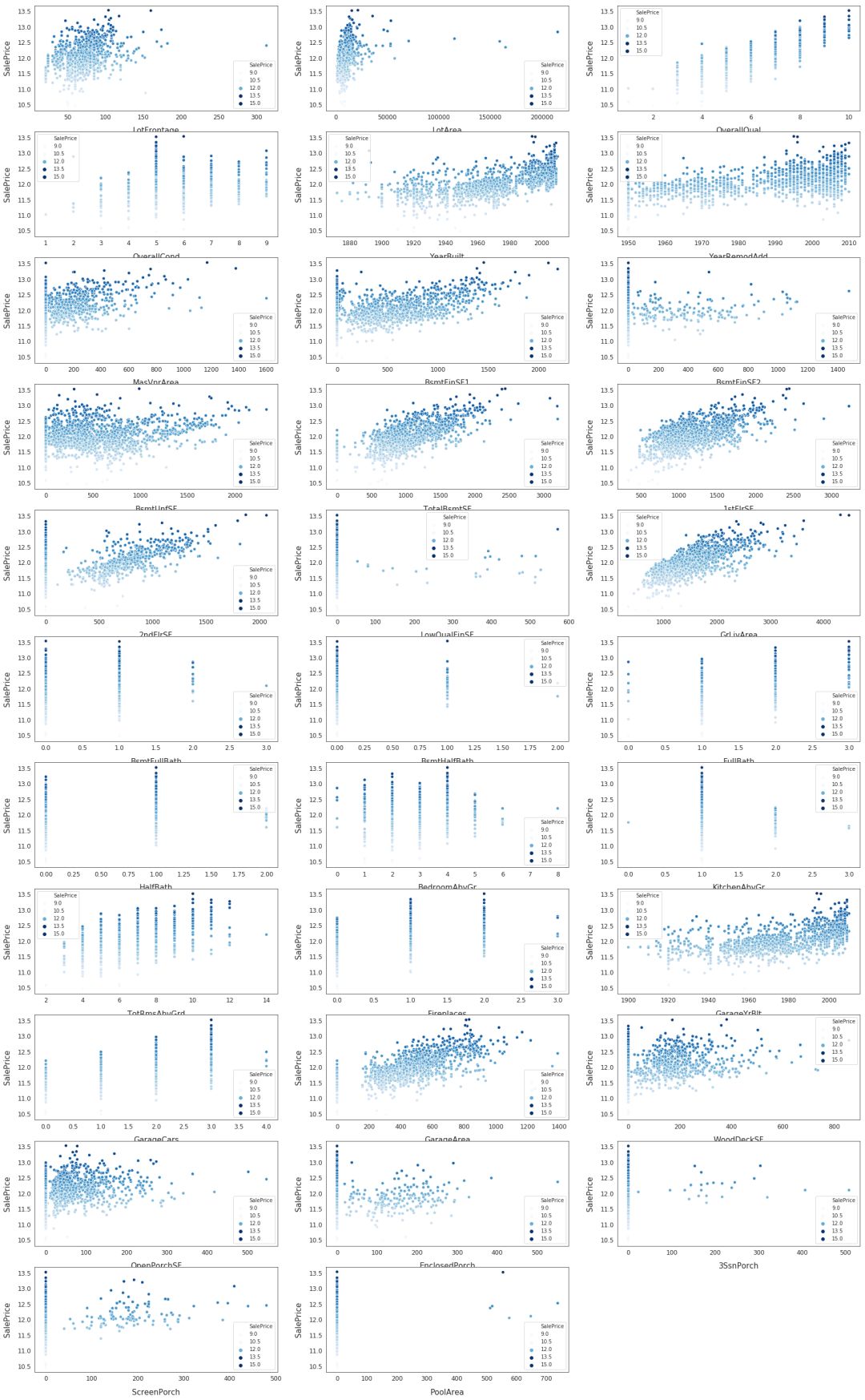
模型训练
模型训练过程中的重要细节
交叉验证:使用12-折交叉验证
模型:在每次交叉验证中,同时训练七个模型(ridge, svr, gradient boosting, random forest, xgboost, lightgbm regressors)
Stacking 方法:使用xgboot训练了元 StackingCVRegressor 学习器
模型融合:所有训练的模型都会在不同程度上过拟合,因此,为了做出最终的预测,将这些模型进行了融合,得到了鲁棒性更强的预测结果
初始化交叉验证,定义误差评估指标
# Setup cross validation folds
kf = KFold(n_splits=12, random_state=42, shuffle=True)
# Define error metrics
def rmsle(y, y_pred): return np.sqrt(mean_squared_error(y, y_pred)) def cv_rmse(model, X=X): rmse = np.sqrt(-cross_val_score(model, X, train_labels, scoring="neg_mean_squared_error", cv=kf)) return (rmse)建立模型
# Light Gradient Boosting Regressor
lightgbm = LGBMRegressor(objective='regression',	num_leaves=6,	learning_rate=0.01,	n_estimators=7000,	max_bin=200,	bagging_fraction=0.8,	bagging_freq=4,	bagging_seed=8,	feature_fraction=0.2,	feature_fraction_seed=8,	min_sum_hessian_in_leaf = 11,	verbose=-1,	random_state=42)	# XGBoost Regressor
xgboost = XGBRegressor(learning_rate=0.01,	n_estimators=6000,	max_depth=4,	min_child_weight=0,	gamma=0.6,	subsample=0.7,	colsample_bytree=0.7,	objective='reg:linear',	nthread=-1,	scale_pos_weight=1,	seed=27,	reg_alpha=0.00006,	random_state=42)	# Ridge Regressor
ridge_alphas = [1e-15, 1e-10, 1e-8, 9e-4, 7e-4, 5e-4, 3e-4, 1e-4, 1e-3, 5e-2, 1e-2, 0.1, 0.3, 1, 3, 5, 10, 15, 18, 20, 30, 50, 75, 100]
ridge = make_pipeline(RobustScaler(), RidgeCV(alphas=ridge_alphas, cv=kf))	# Support Vector Regressor
svr = make_pipeline(RobustScaler(), SVR(C= 20, epsilon= 0.008, gamma=0.0003))	# Gradient Boosting Regressor
gbr = GradientBoostingRegressor(n_estimators=6000,	learning_rate=0.01,	max_depth=4,	max_features='sqrt',	min_samples_leaf=15,	min_samples_split=10,	loss='huber',	random_state=42)	# Random Forest Regressor
rf = RandomForestRegressor(n_estimators=1200,	max_depth=15,	min_samples_split=5,	min_samples_leaf=5,	max_features=None,	oob_score=True,	random_state=42)	# Stack up all the models above, optimized using xgboost
stack_gen = StackingCVRegressor(regressors=(xgboost, lightgbm, svr, ridge, gbr, rf),	meta_regressor=xgboost,	use_features_in_secondary=True)
训练模型
计算每个模型的交叉验证的得分
scores = {}	score = cv_rmse(lightgbm)
print("lightgbm: {:.4f} ({:.4f})".format(score.mean(), score.std()))
scores['lgb'] = (score.mean(), score.std())
lightgbm: 0.1159 (0.0167)
score = cv_rmse(xgboost)
print("xgboost: {:.4f} ({:.4f})".format(score.mean(), score.std()))
scores['xgb'] = (score.mean(), score.std())
xgboost: 0.1364 (0.0175)
score = cv_rmse(svr)
print("SVR: {:.4f} ({:.4f})".format(score.mean(), score.std()))
scores['svr'] = (score.mean(), score.std())
SVR: 0.1094 (0.0200)
score = cv_rmse(ridge)
print("ridge: {:.4f} ({:.4f})".format(score.mean(), score.std()))
scores['ridge'] = (score.mean(), score.std())
ridge: 0.1101 (0.0161)
score = cv_rmse(rf)
print("rf: {:.4f} ({:.4f})".format(score.mean(), score.std()))
scores['rf'] = (score.mean(), score.std())
rf: 0.1366 (0.0188
score = cv_rmse(gbr)
print("gbr: {:.4f} ({:.4f})".format(score.mean(), score.std()))
scores['gbr'] = (score.mean(), score.std())
gbr: 0.1121 (0.0164)
拟合模型
print('stack_gen')
stack_gen_model = stack_gen.fit(np.array(X), np.array(train_labels))
stack_gen
print('lightgbm')
lgb_model_full_data = lightgbm.fit(X, train_labels)
lightgbm
print('xgboost')
xgb_model_full_data = xgboost.fit(X, train_labels)
xgboost
print('Svr')
svr_model_full_data = svr.fit(X, train_labels)
Svr
print('Ridge')
ridge_model_full_data = ridge.fit(X, train_labels)
Ridge
print('RandomForest')
rf_model_full_data = rf.fit(X, train_labels)
RandomForest
print('GradientBoosting')
gbr_model_full_data = gbr.fit(X, train_labels)
GradientBoosting
融合各个模型,并进行最终预测
# Blend models in order to make the final predictions more robust to overfitting
def blended_predictions(X):	return ((0.1 * ridge_model_full_data.predict(X)) + \	(0.2 * svr_model_full_data.predict(X)) + \	(0.1 * gbr_model_full_data.predict(X)) + \	(0.1 * xgb_model_full_data.predict(X)) + \	(0.1 * lgb_model_full_data.predict(X)) + \	(0.05 * rf_model_full_data.predict(X)) + \	(0.35 * stack_gen_model.predict(np.array(X))))
# Get final precitions from the blended model
blended_score = rmsle(train_labels, blended_predictions(X))
scores['blended'] = (blended_score, 0)
print('RMSLE score on train data:')
print(blended_score)
RMSLE score on train data:
0.07537440195302639
各模型性能比较
# Plot the predictions for each model
sns.set_style("white")
fig = plt.figure(figsize=(24, 12))	ax = sns.pointplot(x=list(scores.keys()), y=[score for score, _ in scores.values()], markers=['o'], linestyles=['-'])
for i, score in enumerate(scores.values()):	ax.text(i, score[0] + 0.002, '{:.6f}'.format(score[0]), horizontalalignment='left', size='large', color='black', weight='semibold')	plt.ylabel('Score (RMSE)', size=20, labelpad=12.5)
plt.xlabel('Model', size=20, labelpad=12.5)
plt.tick_params(axis='x', labelsize=13.5)
plt.tick_params(axis='y', labelsize=12.5) plt.title('Scores of Models', size=20) plt.sho 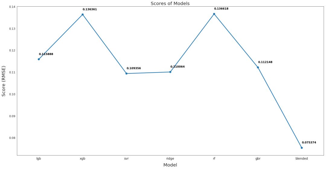
从上图可以看出,融合后的模型性能最好,RMSE 仅为 0.075,该融合模型用于最终预测。
提交预测结果
# Read in sample_submission dataframe
submission = pd.read_csv("../input/house-prices-advanced-regression-techniques/sample_submission.csv")
submission.shape
(1459, 2)
# Append predictions from blended models
submission.iloc[:,1] = np.floor(np.expm1(blended_predictions(X_test)))	# Fix outleir predictions
q1 = submission['SalePrice'].quantile(0.0045)
q2 = submission['SalePrice'].quantile(0.99)
submission['SalePrice'] = submission['SalePrice'].apply(lambda x: x if x > q1 else x*0.77)
submission['SalePrice'] = submission['SalePrice'].apply(lambda x: x if x < q2 else x*1.1)
submission.to_csv("submission_regression1.csv", index=False)
# Scale predictions
submission['SalePrice'] *= 1.001619
submission.to_csv("submission_regression2.csv", index=False)原文链接:
https://www.kaggle.com/lavanyashukla01/how-i-made-top-0-3-on-a-kaggle-competition
(*本文为 AI科技大本营翻译文章,转载请联系 1092722531)
◆
精彩推荐
◆
“只讲技术,拒绝空谈!”2019 AI开发者大会将于9月6日-7日在北京举行,这一届AI开发者大会有哪些亮点?一线公司的大牛们都在关注什么?AI行业的风向是什么?2019 AI开发者大会,倾听大牛分享,聚焦技术实践,和万千开发者共成长。
目前,大会盲订票限量发售中~扫码购票,领先一步!

推荐阅读
干货 | 20个教程,掌握时间序列的特征分析(附代码)
从发展滞后到不断突破,NLP已成为AI又一燃爆点?
长点心吧年轻人,利率不是这么算的!我用Python告诉你亏了多少!
一文看懂数据清洗:缺失值、异常值和重复值的处理
Libra 骗局来了! 受害者会是你吗?
那个裸辞的程序员,后来怎么样了?
FreeWheel是一家怎样的公司?| 人物志
Mac 被曝存在恶意漏洞:黑客可随意调动摄像头,波及四百万用户!
文末送书啦!| Device Mapper,那些你不知道的Docker核心技术
 你点的每个“在看”,我都认真当成了喜欢
相关文章:

JavaBean规范
2019独角兽企业重金招聘Python工程师标准>>> (1)JavaBean 类必须是一个公共类,并将其访问属性设置为 public (2)JavaBean 类必须有一个空的构造函数:类中必须有一个不带参数的公用构造器&#x…

vigra1.8.0的使用
VIGRA stands for "Vision with Generic Algorithms". Its a novel computer vision library that puts its main emphasis oncustomizablealgorithms and data structures. 1、首先,从http://hci.iwr.uni-heidelberg.de/vigra/下载最新源代码࿰…
17个Python小窍门
python中相对不常见却很实用的小窍门。 空谈不如来码代码吧: 交换变量值 给列表元素创建新的分隔符 找列表中出现次数最多的元素 核对两个字符是否为回文 反向输出字符串 反向输出列表 转置2维数组 链式比较 我刚整理了一套2018最新的0基础入门和进阶教程࿰…

用产品思路建设中台,这走得通吗?| 白话中台
作者 | 王健,ThoughtWorks首席咨询师。 十多年国内外大型企业软件设计开发,团队组织转型经验。一直保持着对技术的热爱,热衷于技术分享。目前专注在企业平台化转型、中台战略规划,微服务架构与实施,大型遗留系统服务化…
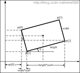
利用cvMinAreaRect2求取轮廓最小外接矩形
转自:http://blog.csdn.net/mine1024/article/details/6044856 对给定的 2D 点集,寻找最小面积的包围矩形,使用函数: CvBox2D cvMinAreaRect2( const CvArr* points, CvMemStorage* storageNULL ); points 点序列或点集数组 …
电脑开机显示Invalidsystemdisk
开机或重启无法进入系统,并在屏幕上显示Invalidsystemdisk,Replacethediskandthenpressanykey或者diskerror之类的字样,这是怎么回事,该如何解决?今天u大师就为大家解决下。 出现这个原因是因为现在的电脑没有可以启…
Windows7 64位下vs2008配置OpenCV2.3.1
1、下载OpenCV2.3.1:http://www.opencv.org.cn/index.php/Download; 2、下载后解压缩:OpenCV-2.3.1-win-superpack.exe,生成一个opencv文件夹; 3、下载CMake:http://www.cmake.org/cmake/resources/softw…
腾讯拥抱开源:首次公布开源路线图,技术研发向共享、复用和开源迈进
整理 | 夕颜出品 | AI科技大本营(ID:rgznai100)导读:去年,知乎上一篇讨论腾讯技术的帖子异常火爆,讨论的主题是当下(2018 年)腾讯的技术建设是否处于落后同体量公司的状态,这篇帖子得…
Babylon.js 3.3发布:更强大的粒子系统和WebVR支持
Babylon.js 3.3版本利用微软混合现实工具包(MRTK)的功能来改进WebVR开发,并改进了其粒子系统控件。 MRTK提供了一系列脚本和组件来加速混合现实应用程序的开发。为了简化GUI VR构建,Bablyon.js利用3D体积网格来布局VR场景的界面&a…

基于Erlang语言的视频相似推荐系统 | 深度
作者丨gongyouliu来源 | 转载自大数据与人工智能(ID:ai-big-data)【导语】:作者在上一篇文章《基于内容的推荐算法》中介绍了基于内容的推荐算法的实现原理。在本篇文章中作者会介绍一个具体的基于内容的推荐算法的实现案例。该案例是作者在2…
MinGW简介
转自:http://baike.baidu.com/view/98554.htm MinGW是指只用自由软件来生成纯粹的Win32可执行文件的编译环境,它是Minimalist GNU on Windows的略称。这里的“纯粹”是指使用msvcrt.dll的应用程序。无法使用MFC (Microsoft Foundation Classes微软基础类…
Confluence 6 创建小组的公众空间
2019独角兽企业重金招聘Python工程师标准>>> 现在是我们可以开始创建公众空间的时候了,全世界都希望知道这个项目和勇敢的探险活动。 在这个步骤中,我们将会创建一个项目小组的空间,并且将这个空间公布给全世界。这个表示的是你将…
windows 7 可以清除的文件
缓解系统磁盘空间不足的情况1、系统盘根目录下的MSOCache是office的安装备份文件,可以删除。2、c:\user\用户名\appdate\local\temp是软件安装时留下的临时文件。3、c:\windows\SoftwareDistribution中存放的是系统补丁更新包及旧的系统文件。4、c:\windows\winsxs\…
阿里最新论文解读:考虑时空域影响的点击率预估模型DSTN
作者 | 石晓文转载自小小挖掘机(ID: wAIsjwj)【导语】:在本文中,阿里的算法人员同时考虑空间域信息和时间域信息,来进行广告的点击率预估。什么是时空域?我们可以分解为空间域(spatial domain)和时间域(tem…
windows7 64位机上配置MinGW+Codeblocks+ wxWidgets
在Windows7 64位机子上安装配置MinGWCodeblockswxWidgets步骤如下: 1、 下载mingw-get-inst-20111118:http://sourceforge.net/projects/mingw/; 2、 双击mingw-get-inst-20111118.exe,一般按默认即可,选择自己需要…

jQuery带动画的弹出对话框
在线演示 本地下载
陶哲轩实分析 习题 13.4.6
设 $(X,d)$ 是度量空间,并设 $(E_{\alpha})_{\alpha\in I}$ 是 $X$ 中的一族连通集合.还设 $\bigcap_{\alpha\in I}E_{\alpha}$ 不空.证明 $\bigcup_{\alpha\in I}E_{\alpha}$ 是连通的.证明:由于 $\bigcap_{\alpha\in I}E_{\alpha}$ 是不空的,因此存在 $p\in \bigcap_{\alpha\…
一年参加一次就够,全新升级的AI开发者大会议程出炉!
“只讲技术,拒绝空谈”的AI开发者大会再次来临!2018 年的AI开发者大会,作为年度人工智能领域面向专业开发者的一次高规格技术盛会,上千名开发者与上百名技术专家齐聚一堂,大会以“AI技术与应用”为核心,就人…
Windows7下配置MinGW+CodeBlocks+OpenCV2.3.1
1、下载mingw-get-inst-20111118:http://sourceforge.net/projects/mingw/; 2、双击mingw-get-inst-20111118.exe,一般按默认即可,选择自己需要的组件; 3、添加MinGW环境变量:选择计算机-->点击右键--…
Spark SQL基本操作以及函数的使用
2019独角兽企业重金招聘Python工程师标准>>> 引语: 本篇博客主要介绍了Spark SQL中的filter过滤数据、去重、集合等基本操作,以及一些常用日期函数,随机函数,字符串操作等函数的使用,并列编写了示例代码&am…
OpenCV提取轮廓(去掉面积小的轮廓)
转自:http://www.kaixuela.net/?p23 #include <stdio.h> #include "cv.h" #include "cxcore.h" #include "highgui.h" #include <iostream> using namespace std; #pragma comment(lib,"cv.lib") #pra…
软工作业 5:词频统计——增强功能
一、基本信息 1.1 编译环境、项目名称、作者 1 #编译环境:python3.6 2 #项目名称:软工作业5-词频统计—增强功能 3 #作者:1613072055 潘博 4 # 1613072056 侯磊 1.2项目地址 本次作业地址: https://www.cnblogs.com/panboo/项目git地址: https://g…
Linux之文件权限管理
chmod ux转载于:https://www.cnblogs.com/chaoren399/archive/2013/03/11/2953727.html
如果三十年前有这些AI技术,可可西里的悲剧不会发生
作者 | 神经小姐姐来源 | HyperAI超神经(ID:HyperAI)而被盗猎者大量的非法捕杀。多种野生动物都处于濒临灭绝的局面,人工智能等技术,能够在帮助保护野生动物上,发挥比较大的作用,让我们能够生存…
Percona-Server-5.5.30安装
1、安装系统环境 yum install -y gcc gcc-c autoconf automake zlib* libxml* ncurses-devel libmcrypt* libtool-ltdl-devel* cmake bison 2、下载源码包 1 http://www.percona.com/downloads/ 2 3 wget -c http://www.percona.com/redir/downloads/Percona-Server-5.5/Perc…
OpenCV中SVM的使用
转自:http://download.csdn.net/download/gaogaogao124/3125857 略有改动: #include"stdafx.h" #include<opencv2/opencv.hpp> #include<cmath> #include<ctime> using namespace std; int _tmain(int argc,_TCHAR…
数据不够,用GAN来凑!
作者 | CV君来源 | 我爱计算机视觉(ID:aicvml)在计算机视觉领域,深度学习方法已全方位在各个方向获得突破,这从近几年CVPR 的论文即可看出。但这往往需要大量的标注数据,比如最著明的ImageNet数据集&#x…
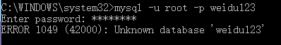
MySQL的登陆错误:ERROR 1049 (42000): Unknown database 'root'
刚刚装上数据库的时候,直接按照这个格式就登陆上去了,突然莫名其妙登陆不上去了 但是现在突然死活登陆不上去了 于是拿着这个报错信息在网上找啊找,终于找了了错误的原因 -p和密码是连在一起的,赶紧一试,果然可以登陆&…

分布式缓存系统Memcached简介与实践
缘起: 在数据驱动的web开发中,经常要重复从数据库中取出相同的数据,这种重复极大的增加了数据库负载。缓存是解决这个问题的好办法。但是ASP.NET中的虽然已经可以实现对页面局部进行缓存,但还是不够灵活。此时Memcached或许是你想要的。Memca…
Windows7 libsvm库中grid.py的使用步骤
1、从http://www.csie.ntu.edu.tw/~cjlin/libsvm/下载最新的libsvm-3.12库(libsvm-3.12.tar.gz或libsvm-3.12.zip),将其放到F:\libsvm文件夹下解压缩,生成一个libsvm-3.12文件夹; 2、从http://www.gnuplot.info/下载最新的gnuplot即gp460-wi…