【Smooth】非线性优化
文章目录
- 非线性优化
- 0 .case实战
- 0.1求解思路
- 0.2 g2o求解
- 1. 状态估计问题
- 1.1 最大后验与最大似然
- 1.2 最小二乘的引出
- 2. 非线性最小二乘
- 2.1 一阶和二阶梯度法
- 2.2 高斯牛顿法
- 2.2 列文伯格-马夸尔特方法(阻尼牛顿法)
- 3 Ceres库的使用
- 4 g2o库的使用
非线性优化
0 .case实战
0.1求解思路
对两幅图像img_1,img_2分别提取特征点
特征匹配
通过depth,获得第一幅图像匹配的特征点的深度,由相机内参K恢复这些特征点的三维坐标(相机坐标系)。
由第一幅图像中的特征点的三维坐标、第二幅图像中特征点的2D像素坐标,以及相机内参K作为优化函数的输入,分别采用如下方法进行优化
牛顿高斯法
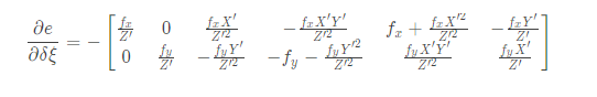
(1)构建误差方程,由相机位姿、相机内参获得第一幅图像特征点对应的三维坐标到第二幅图像中的投影(像素坐标),与真实提取的第二幅图像中特征点的像素坐标作差即重投影误差:
(2)关于相机位姿李代数的一阶变化:雅可比矩阵
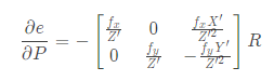
(3)误差关于空间点位置的导数(在这个实例代码中没用上,仅对位姿做了优化,并没有优化空间点位置):
(4)构建增量方程,g=-J(x)f(x),代码中g对应e。
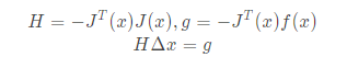
(5)LDLT分解,求增量方程
dx = H.ldlt().solve(b)。
(6)更新变量pose = Sophus::SE3d::exp(dx) * pose。
(7)在新的位姿下,进行新一轮迭代,重复(1)-(7)。0.2 g2o求解
构建定点(顶点代表优化变量),在3D2D的PnP位姿求解中,仅优化了位姿。
(1)顶点(变量)_estimate = Sophus::SE3d();
(2)变量更新_estimate = Sophus::SE3d::exp(update_eigen) * _estimate;(1)边连接的顶点(在这里只有一个顶点,即相机位姿),边为误差项,即由顶点引起的误差
const VertexPose *v = static_cast<VertexPose *> (_vertices[0]);
Sophus::SE3d T = v->estimate();
Eigen::Vector3d pos_pixel = _K * (T * _pos3d);
pos_pixel /= pos_pixel[2];
_error = _measurement - pos_pixel.head<2>();
(2)误差对顶点求导,得到
_jacobianOplusXig2o的库调用过程
增加顶点optimizer.addVertex(vertex_pose);
增加边(是一个循环,每一个特征点就有一条边):optimizer.addEdge(edge);
初始化optimizer.initializeOptimization();
求解optimizer.optimize(10);
获取结果:pose = vertex_pose->estimate();
1. 状态估计问题
1.1 最大后验与最大似然
- 经典 SLAM 模型:
\left{\begin{array}{c}
x_{k}=f\left(x_{k-1}, u_{k}\right)+w_{k} \
z_{k, j}=f\left(y_{j}, x_{k}\right)+v_{k, j}
\end{array}\right.
其中x{k}为相机的位姿,u为输入数据,即为采集到的数据
假如我们在x{k} 处观测到路标 y_{j} 对应到图像上的像素位置 z_{k, j}, 那么我们的观测方程可以表示为:
s z_{k, j}=K \exp \left(\xi^{\wedge}\right) y_{i}
- 在运动和观测方程中,通常假设两个噪声项 w_{k}, v_{k} 满足零均值的高斯分布:
w_{k} N\left(0, R_{k}\right), v_{k} N\left(0, Q_{k, j}\right)
- 状态估计问题:通过带噪声的数据 z和u , 推断位姿 x和地图y (以及它们的概率分布),其中有优化方法有:
(1)扩展卡尔曼滤波器(EKF)求解,关心的是当前时刻的状态估计,而对直之前的状态没有多加考虑。
(2)非线性优化,使用所有时刻采集到的数据进行状态估计,被认为优于传统滤波器,成为当前视觉slam的主流。
非线性优化把所待估计的变量都放在一个状态变量中:
x=\left{x_{1}, \ldots, x_{N}, y_{1}, \ldots, y_{M}\right}
已知:输入读数u,观测值z。(带噪声)
目标: P(x \mid z, u),只考虑z时:P(x \mid z)
贝叶斯法则:
P(x \mid z)=\frac{P(z \mid x) P(x)}{P(z)} \rightarrow P(z \mid x) P(x)
贝叶斯法则左侧通常称为后验概率。它右侧的 P(z \mid x) 称为似然,另一部分P ( x ) 称为先验
直接求后验分布较困难,转而求一个状态最优估计,使得在该状态下,后验概率最大化(MPA):
x^{*} M A P=\operatorname{argmax} P(x \mid z)=\operatorname{argmax} P(z)
若不知道机器人位姿大概在什么地方,此时就没有了先验。进而可以求解x x*x*的最大似然估计:
x_{M L E}^{*}=\operatorname{argmax} P(z \mid x)
最大似然估计,可以理解成:“**在什么样的状态下,最可能产生现在观测到的数据**”
1.2 最小二乘的引出
- 对于某一次观测:
z_{k, j}=h\left(y_{j}, x_{k}\right)+v_{k, j}
假设噪声项 v_{k} \sim N\left(0, Q_{k, j}\right), 所以观测数据的条件概率为:
P\left(z_{k, j} \mid x_{k}, y_{j}\right)=N\left(h\left(y_{i}, x_{k}\right), Q_{k, j}\right)
- 为了计算使它最大化的 x_{k}, y_{k},使用最小化负对数的方式,来求一个高斯分布的最大似然。考虑一个任意的高维高斯分布v_{k} \sim N(\mu, \Sigma), 它的概率密度函数展开形式为:
P(x)=\frac{1}{\sqrt{(2 \pi)^{N} \operatorname{det}\left(\sum\right)}} \exp \left(-\frac{1}{2}(x-\mu)^{T} \Sigma^{-1}(x-\mu)\right)
**取负对数:**
-\ln (P(x))=\frac{1}{2} \ln \left((2 \pi)^{N} \operatorname{det}(\Sigma)\right)+\frac{1}{2}(x-\mu)^{T} \Sigma^{-1}(x-\mu)
- 第一项与 x 无关,可以略去。代入 SLAM 的观测模型,相当于在求:
x^{*}=\operatorname{argmin}\left(\left(z_{k, j}-h\left(x_{k}, y_{j}\right)\right)^{T} Q_{k, j}^{-1}\left(z_{k, j}-h\left(x_{k}, y_{j}\right)\right)\right)
该式等价于最小化噪声项(即误差)的平方(Σ ΣΣ 范数意义下)
- 对于所有的运动和任意的观测,定义数据与估计值之间的误差:
\begin{array}{c}
e_{v, k}=x_{k}-f\left(x_{k-1}, u_{k}\right) \
e_{v, j, k}=z_{k, j}-f\left(x_{k}, y\right)
\end{array}
并求该误差的平方之和:
J(x)=\sum_{k} e_{T}^{v, k} R_{k}^{-1} e_{v, k}+\sum_{k} \sum_{j} e_{y, k, j}^{T} Q_{k, j}^{-1} e_{y, k, j}
这样就得到一个总体意义下的最小二乘问题,它的最优解等价于状态的最大似然估计。由于噪声的存在,当我们把估计的轨迹与地图代入SLAM的运动、观测方程时,并不会很完美,可以对状态进行微调,使得整体的误差下降到一个极小值。
- SLAM中的最小二乘问题具有一些特定的结构:
(1)整个问题的目标函数由许多个误差的(加权的)平方和组成。虽然总体的状态变量维数很高,但每个误差项都是简单的,仅与一俩个状态变量有关,运动误差只与x_{k-1}, x_{k} 有关,观测误差只与 x_{k}, y_{j} 有关,每个误差是个小规模约束,把这误差项的小雅克比矩阵放在整体的雅克比矩阵中。称每个误差项对应优化变量为参数快。
整体误差由很多小误差项之和组成的问题,其增量方程具有一定的稀疏性。
(2)如果使用李代数表示,那么该问题转换成**无约束最小二乘问题*,用旋转矩阵描述姿态会引入自身的约束
(3)使用二范数度量误差,相当于欧式空间中距离的平方。
2. 非线性最小二乘
最简单的最小二乘问题:
\min {x} \frac{1}{2}|f(x)|{2}^{2}
为求其最小值,则需要求其导数,然后得到其求解 x的最优解
对于不方便求解的最小二乘问题,可以用迭代的方法,从初始值出发,不断的跟新当前的优化变量,使目标函数下降,具体步骤有:
(1)给定某个初始值。
(2)对于第k次迭代,寻找增量 \Delta x_{k} , 使得 f\left(x_{k}+\Delta x_{k}\right) |_{2}^{2} 这里应该是二范数)达到最小。
(3)若\Delta x_{k}足够小,则停止。
(4)否则,令x_{k+1}=x_{k}+\Delta x_{k} 返回第2步。
2.1 一阶和二阶梯度法
将目标函数在 x xx 附近进行泰勒展开:
|f(x+\Delta x)|{2}^{2} \approx|f(x)|{2}^{2}+J(x) \Delta x+\frac{1}{2} \Delta x^{T} H \Delta x
J是|f(x)|_{2}^{2} 关于x xx的导数(雅克比矩阵),H HH是二阶导数(海塞矩阵)
最速梯度下降法:只保留一阶梯度,增量的方向为:
\Delta x{*}=-J{I}(x)
- 牛顿法:保留二阶梯度,增量方程为:
\Delta x{*}=-J{I}(x)\Delta x{*}=\operatorname{argmin}|f(x)|_{2}{2}+J(x) \Delta x+\frac{1}{2} x^{T} H \Delta x
求右侧等式关于 ∆x的导数并令它为零,得到了增量的解:
H \Delta X=-J^{T}
- 两种方法的问题:
(1)最速下降法过于贪心,容易走出锯齿路线,反而增加了迭代次数。
(2)牛顿法则需要计算目标函数的 H矩阵,这在问题规模较大时非常困难,通常倾向于避免 H 的计算。
2.2 高斯牛顿法
- 高斯牛顿法,它的思想是将f(x) 进行泰勒展开(目标函数不是f(x) )
f(x+\Delta x) \approx f(x)+J(x) \Delta x
f(J) 是一个m ∗ n mnm∗n*雅克比矩阵,当前的目标是为了寻找下降矢量 ∆x,使得 \left|f(x+\Delta x)^{2}\right| 达到最小。
- 为了求 \Delta x_{k} 需要解一个线性的最小二乘问题
\Delta x^{*}=\arg \min _{\Delta x} \frac{1}{2}|f(x)+J(x) \Delta x|^{2}
考虑的是 \Delta x_{k} 的导数(而不是x x*x*) ,先展开目标函数的平方项
\begin{array}{c}
\frac{1}{2}|f(x)+J(x) \Delta x|^{2}=\frac{1}{2}(f(x)+J(x) \Delta x)^{T}(f(x)+J(x) \Delta x) \
\left.=\frac{1}{2}(|f(x)|)_{2}^{2}+2 f(x)^{T} J(x) \Delta x+\Delta x J(x)^{T} J(x) \Delta x\right)
\end{array}
上式关于\Delta x的导数,并令其为零:
J(x)^{T} J(x) \Delta x=-J(x)^{T} f(x)
这个方程称之为增量方程,也称之为高斯牛顿方程或正规方程,将左边的系数设为H,右边的系数设为g ,则有
H \Delta x=g
- 高斯牛顿法求解的算法步骤可写成:
(1)给定初始值x_{0}
(2)对于第k 次迭代,求出当前的雅克比矩阵J\left(x_{k}\right) 和误差 f\left(x_{k}\right)(3)求解增量方程: H \Delta x_{k}=g(4)若\Delta x 足够小,则停止。否则,令 x_{k+1}=x_{k}+\Delta x_{k} 返回第二步
- 高斯牛顿法的缺点:
(1)要求H 是可逆的,而且是正定的,如果出现H 矩阵奇异或者病态,此时增量的稳定性较差,导致算法不收敛
(2)步长问题,若求出来的 \Delta x_{k}太长,则可能出现局部近似不够准确,无法保证迭代收敛。
2.2 列文伯格-马夸尔特方法(阻尼牛顿法)
信赖区域方法 (Trust Region Method):给 \Delta x添加一个信赖区域(Trust Region),不能让它太大而使得近似不准确
考虑使用如下公式来判断泰勒近似是否够好
\rho=\frac{f(x+\Delta x)-\Delta x}{J(x) \Delta x}
(1)如果 ρ ρρ 接近于 1,则近似是好的。
(2)如果 ρ ρρ太小,说明实际减小的值远少于近似减小的值,则认为近似比较差,需要缩小近似范围。
(3)如果 ρ ρρ 比较大,则说明实际下降的比预计的更大,我们可以放大近似范围。
- 改良版的非线性优化框架
[外链图片转存失败,源站可能有防盗链机制,建议将图片保存下来直接上传(img-i5um1muo-1610464509672)(C:\Users\guoqi\AppData\Roaming\Typora\typora-user-images\1610039803776.png)]
- 由于是有约束优化,可以利用拉格朗日乘子将其转化为一个无约束优化问题:
\min {\Delta x{k}} \frac{1}{2}\left|f\left(x_{k}+J\left(x_{k} \Delta x_{k}\right)\right)\right|^{2}+\frac{\lambda}{2}|D \Delta x|^{2}
类似高斯牛顿法展开,可得其增量的线性方程:
\left(H+\lambda D^{T} D\right) \Delta X=g
考虑它的简化形式,即D=I,那么相当于求解:
(H+\lambda I) \Delta x=g
(1)当参数λ λ*λ*较小时,H 占主导地位,说明二次近似模型在该范围内是比较好的,该方法接近于高斯牛顿法。
(2)当参数λ λλ较大时,列文伯格-马夸尔特方法接近于一阶梯度下降法,说明二次近似不好。
(3)该方法可在一定程度上避免线性方程组的系数矩阵的非奇异和病态问题),提供更稳定、更准确的增量\Delta x。
- 非线性优化的框架分为Line Search和Trust Region两类。
(1)Line Search:先固定搜索方向,后寻找步长,以最速梯度法和高斯牛顿法为代表。
(2)Trust Region:先固定搜索区域,再考虑找该区域的最优点,以列文伯格-马夸尔特方法为代表
3 Ceres库的使用
ceres库的使用教程这份google的资料很详细,足够解决我们遇到的问题。
ceres example 见链接。
3.1 实例
#include <iostream>
#include <opencv2/core/core.hpp>
#include <opencv2/features2d/features2d.hpp>
#include <opencv2/highgui/highgui.hpp>
#include <opencv2/calib3d/calib3d.hpp>
#include <Eigen/Core>
#include <Eigen/Geometry>
#include <chrono>
#include <ceres/ceres.h>
#include <ceres/rotation.h>
using namespace std;
using namespace cv;void find_feature_matches ( const Mat& img_1, const Mat& img_2,std::vector<KeyPoint>& keypoints_1,std::vector<KeyPoint>& keypoints_2,std::vector< DMatch >& matches )
{//-- 初始化Mat descriptors_1, descriptors_2;// used in OpenCV3Ptr<FeatureDetector> detector = ORB::create();Ptr<DescriptorExtractor> descriptor = ORB::create();// use this if you are in OpenCV2// Ptr<FeatureDetector> detector = FeatureDetector::create ( "ORB" );// Ptr<DescriptorExtractor> descriptor = DescriptorExtractor::create ( "ORB" );Ptr<DescriptorMatcher> matcher  = DescriptorMatcher::create ( "BruteForce-Hamming" );//-- 第一步:检测 Oriented FAST 角点位置detector->detect ( img_1,keypoints_1 );detector->detect ( img_2,keypoints_2 );//-- 第二步:根据角点位置计算 BRIEF 描述子descriptor->compute ( img_1, keypoints_1, descriptors_1 );descriptor->compute ( img_2, keypoints_2, descriptors_2 );//-- 第三步:对两幅图像中的BRIEF描述子进行匹配,使用 Hamming 距离vector<DMatch> match;// BFMatcher matcher ( NORM_HAMMING );matcher->match ( descriptors_1, descriptors_2, match );//-- 第四步:匹配点对筛选double min_dist=10000, max_dist=0;//找出所有匹配之间的最小距离和最大距离, 即是最相似的和最不相似的两组点之间的距离for ( int i = 0; i < descriptors_1.rows; i++ ){double dist = match[i].distance;if ( dist < min_dist ) min_dist = dist;if ( dist > max_dist ) max_dist = dist;}printf ( "-- Max dist : %f \n", max_dist );printf ( "-- Min dist : %f \n", min_dist );//当描述子之间的距离大于两倍的最小距离时,即认为匹配有误.但有时候最小距离会非常小,设置一个经验值30作为下限.for ( int i = 0; i < descriptors_1.rows; i++ ){if ( match[i].distance <= max ( 2*min_dist, 30.0 ) ){matches.push_back ( match[i] );}}
}Point2d pixel2cam ( const Point2d& p, const Mat& K )
{return Point2d(( p.x - K.at<double> ( 0,2 ) ) / K.at<double> ( 0,0 ),( p.y - K.at<double> ( 1,2 ) ) / K.at<double> ( 1,1 ));
}//Eigen::Matrix<double,3,3> camera_matrix;
//camera_matrix <<520.9, 0, 325.1, 0, 521.0, 249.7, 0, 0, 1;
Mat K = ( Mat_<double> ( 3,3 ) << 520.9, 0, 325.1, 0, 521.0, 249.7, 0, 0, 1 );struct CurveFittingCost {CurveFittingCost(Point2d point2d, Point3d point3d) : _point2d(point2d), _point3d(point3d) {}template<typename T>bool operator() (const T *const camera_pose,T *residual)const{T point[3];point[0] = T(_point3d.x);point[1] = T(_point3d.y);point[2] = T(_point3d.z);T p[3];ceres::AngleAxisRotatePoint(camera_pose, point, p);p[0] += camera_pose[3]; p[1] += camera_pose[4]; p[2] +=camera_pose[5];//cam2world//p[0] / p[2],p[1] / p[2] is norm coordinate,the real depth id p[2]T x_p = p[0] / p[2];T y_p = p[1] / p[2];                                                 T predicted_x = x_p * K.at<double>(0,0)+K.at<double>(0,2);T predicted_y = y_p * K.at<double>(1,1)+K.at<double>(1,2);residual[0] = T(_point2d.x) - predicted_x;residual[1] = T(_point2d.y) - predicted_y;return true;}static ceres::CostFunction* Create(Point2d point2d, Point3d point3d) {return (new ceres::AutoDiffCostFunction<CurveFittingCost, 2, 6>(new CurveFittingCost(point2d, point3d)));}const Point2d _point2d;const Point3d _point3d;
};int main ( int argc, char** argv )
{if ( argc != 5 ){cout<<"usage: pose_estimation img1 img2 depth1 depth2"<<endl;return 1;}//-- 读取图像Mat img_1 = imread ( argv[1], CV_LOAD_IMAGE_COLOR );Mat img_2 = imread ( argv[2], CV_LOAD_IMAGE_COLOR );vector<KeyPoint> keypoints_1, keypoints_2;vector<DMatch> matches;find_feature_matches ( img_1, img_2, keypoints_1, keypoints_2, matches );cout<<"一共找到了"<<matches.size() <<"组匹配点"<<endl;// 建立3D点Mat d1 = imread ( argv[3], CV_LOAD_IMAGE_UNCHANGED ); // 深度图为16位无符号数,单通道图像Mat K = ( Mat_<double> ( 3,3 ) << 520.9, 0, 325.1, 0, 521.0, 249.7, 0, 0, 1 );vector<Point3f> pts_3d;vector<Point2f> pts_2d;for ( DMatch m:matches ){ushort d = d1.ptr<unsigned short> (int ( keypoints_1[m.queryIdx].pt.y )) [ int ( keypoints_1[m.queryIdx].pt.x ) ];if ( d == 0 )   // bad depthcontinue;float dd = d/5000.0;Point2d p1 = pixel2cam ( keypoints_1[m.queryIdx].pt, K );pts_3d.push_back ( Point3f ( p1.x*dd, p1.y*dd, dd ) );pts_2d.push_back ( keypoints_2[m.trainIdx].pt );std::cout<<"point look "<<std::endl;std::cout<<keypoints_2[m.trainIdx].pt.x<<"  "<<keypoints_2[m.trainIdx].pt.y<<std::endl;std::cout<<p1.x*dd<<"  "<<p1.y*dd<<"   "<< dd <<std::endl;getchar();}double r_x = 1.0, r_y = 1.0, r_z = 1.0;double t_x = 1.0, t_y = 1.0, t_z = 1.0;double camera[6] = { r_x,r_y,r_z,t_x,t_y,t_z};ceres::Problem problem;for (size_t i = 0; i < pts_2d.size(); i++){ceres::CostFunction* cost_function =CurveFittingCost::Create(pts_2d[i],pts_3d[i]);problem.AddResidualBlock(cost_function,nullptr	/* squared loss */,camera);}ceres::Solver::Options options;options.linear_solver_type = ceres::DENSE_SCHUR;options.minimizer_progress_to_stdout = true;ceres::Solver::Summary summary;ceres::Solve(options, &problem, &summary);std::cout << summary.FullReport() << std::endl;std::cout << "**************" << std::endl;Mat R_vec = (Mat_<double>(3, 1) << camera[0], camera[1], camera[2]);std::cout << "camera: " << std::endl;std::cout << camera[0] << " " << camera[1] << " " << camera[2] << std::endl;std::cout << camera[3] << " " << camera[4] << " " << camera[5] << std::endl;std::cout << "**************" << std::endl;Mat R_cvest;Rodrigues(R_vec, R_cvest);//罗德里格斯公式,旋转向量转旋转矩阵std::cout << "R_cvest=" << std::endl << R_cvest << std::endl;Eigen::Matrix3d R_est;Eigen::Vector3d t_est(camera[3], camera[4], camera[5]);std::cout << "t_est=" << std::endl<< t_est << std::endl;std::cout << "**************" << std::endl;Eigen::Isometry3d T(R_est);//构造变换矩阵与输出T.pretranslate(t_est);std::cout << T.matrix() << std::endl;
}
4 g2o库的使用
这里参考高翔博士的代码,举个栗子。详见slambook2 ch7 pose_estimation_2d2d.cpp部分
#include <iostream>
#include <opencv2/core/core.hpp>
#include <opencv2/features2d/features2d.hpp>
#include <opencv2/highgui/highgui.hpp>
#include <opencv2/calib3d/calib3d.hpp>
#include <Eigen/Core>
#include <g2o/core/base_vertex.h>
#include <g2o/core/base_unary_edge.h>
#include <g2o/core/sparse_optimizer.h>
#include <g2o/core/block_solver.h>
#include <g2o/core/solver.h>
#include <g2o/core/optimization_algorithm_gauss_newton.h>
#include <g2o/solvers/dense/linear_solver_dense.h>
#include <sophus/se3.hpp>
#include <chrono>using namespace std;
using namespace cv;void find_feature_matches(const Mat &img_1, const Mat &img_2,std::vector<KeyPoint> &keypoints_1,std::vector<KeyPoint> &keypoints_2,std::vector<DMatch> &matches);// 像素坐标转相机归一化坐标
Point2d pixel2cam(const Point2d &p, const Mat &K);// BA by g2o
typedef vector<Eigen::Vector2d, Eigen::aligned_allocator<Eigen::Vector2d>> VecVector2d;
typedef vector<Eigen::Vector3d, Eigen::aligned_allocator<Eigen::Vector3d>> VecVector3d;void bundleAdjustmentG2O(const VecVector3d &points_3d,const VecVector2d &points_2d,const Mat &K,Sophus::SE3d &pose
);// BA by gauss-newton
void bundleAdjustmentGaussNewton(const VecVector3d &points_3d,const VecVector2d &points_2d,const Mat &K,Sophus::SE3d &pose
);int main(int argc, char **argv) {if (argc != 5) {cout << "usage: pose_estimation_3d2d img1 img2 depth1 depth2" << endl;return 1;}//-- 读取图像Mat img_1 = imread(argv[1], CV_LOAD_IMAGE_COLOR);Mat img_2 = imread(argv[2], CV_LOAD_IMAGE_COLOR);assert(img_1.data && img_2.data && "Can not load images!");vector<KeyPoint> keypoints_1, keypoints_2;vector<DMatch> matches;find_feature_matches(img_1, img_2, keypoints_1, keypoints_2, matches);cout << "一共找到了" << matches.size() << "组匹配点" << endl;// 建立3D点Mat d1 = imread(argv[3], CV_LOAD_IMAGE_UNCHANGED);       // 深度图为16位无符号数,单通道图像Mat K = (Mat_<double>(3, 3) << 520.9, 0, 325.1, 0, 521.0, 249.7, 0, 0, 1);vector<Point3f> pts_3d;vector<Point2f> pts_2d;for (DMatch m:matches) {ushort d = d1.ptr<unsigned short>(int(keypoints_1[m.queryIdx].pt.y))[int(keypoints_1[m.queryIdx].pt.x)];if (d == 0)   // bad depthcontinue;float dd = d / 5000.0;Point2d p1 = pixel2cam(keypoints_1[m.queryIdx].pt, K);pts_3d.push_back(Point3f(p1.x * dd, p1.y * dd, dd));pts_2d.push_back(keypoints_2[m.trainIdx].pt);}cout << "3d-2d pairs: " << pts_3d.size() << endl;chrono::steady_clock::time_point t1 = chrono::steady_clock::now();Mat r, t;solvePnP(pts_3d, pts_2d, K, Mat(), r, t, false); // 调用OpenCV 的 PnP 求解,可选择EPNP,DLS等方法Mat R;cv::Rodrigues(r, R); // r为旋转向量形式,用Rodrigues公式转换为矩阵chrono::steady_clock::time_point t2 = chrono::steady_clock::now();chrono::duration<double> time_used = chrono::duration_cast<chrono::duration<double>>(t2 - t1);cout << "solve pnp in opencv cost time: " << time_used.count() << " seconds." << endl;cout << "R=" << endl << R << endl;cout << "t=" << endl << t << endl;VecVector3d pts_3d_eigen;VecVector2d pts_2d_eigen;for (size_t i = 0; i < pts_3d.size(); ++i) {pts_3d_eigen.push_back(Eigen::Vector3d(pts_3d[i].x, pts_3d[i].y, pts_3d[i].z));pts_2d_eigen.push_back(Eigen::Vector2d(pts_2d[i].x, pts_2d[i].y));}cout << "calling bundle adjustment by gauss newton" << endl;Sophus::SE3d pose_gn;t1 = chrono::steady_clock::now();bundleAdjustmentGaussNewton(pts_3d_eigen, pts_2d_eigen, K, pose_gn);t2 = chrono::steady_clock::now();time_used = chrono::duration_cast<chrono::duration<double>>(t2 - t1);cout << "solve pnp by gauss newton cost time: " << time_used.count() << " seconds." << endl;cout << "calling bundle adjustment by g2o" << endl;Sophus::SE3d pose_g2o;t1 = chrono::steady_clock::now();bundleAdjustmentG2O(pts_3d_eigen, pts_2d_eigen, K, pose_g2o);t2 = chrono::steady_clock::now();time_used = chrono::duration_cast<chrono::duration<double>>(t2 - t1);cout << "solve pnp by g2o cost time: " << time_used.count() << " seconds." << endl;return 0;
}void find_feature_matches(const Mat &img_1, const Mat &img_2,std::vector<KeyPoint> &keypoints_1,std::vector<KeyPoint> &keypoints_2,std::vector<DMatch> &matches) {//-- 初始化Mat descriptors_1, descriptors_2;// used in OpenCV3Ptr<FeatureDetector> detector = ORB::create();Ptr<DescriptorExtractor> descriptor = ORB::create();// use this if you are in OpenCV2// Ptr<FeatureDetector> detector = FeatureDetector::create ( "ORB" );// Ptr<DescriptorExtractor> descriptor = DescriptorExtractor::create ( "ORB" );Ptr<DescriptorMatcher> matcher = DescriptorMatcher::create("BruteForce-Hamming");//-- 第一步:检测 Oriented FAST 角点位置detector->detect(img_1, keypoints_1);detector->detect(img_2, keypoints_2);//-- 第二步:根据角点位置计算 BRIEF 描述子descriptor->compute(img_1, keypoints_1, descriptors_1);descriptor->compute(img_2, keypoints_2, descriptors_2);//-- 第三步:对两幅图像中的BRIEF描述子进行匹配,使用 Hamming 距离vector<DMatch> match;// BFMatcher matcher ( NORM_HAMMING );matcher->match(descriptors_1, descriptors_2, match);//-- 第四步:匹配点对筛选double min_dist = 10000, max_dist = 0;//找出所有匹配之间的最小距离和最大距离, 即是最相似的和最不相似的两组点之间的距离for (int i = 0; i < descriptors_1.rows; i++) {double dist = match[i].distance;if (dist < min_dist) min_dist = dist;if (dist > max_dist) max_dist = dist;}printf("-- Max dist : %f \n", max_dist);printf("-- Min dist : %f \n", min_dist);//当描述子之间的距离大于两倍的最小距离时,即认为匹配有误.但有时候最小距离会非常小,设置一个经验值30作为下限.for (int i = 0; i < descriptors_1.rows; i++) {if (match[i].distance <= max(2 * min_dist, 30.0)) {matches.push_back(match[i]);}}
}Point2d pixel2cam(const Point2d &p, const Mat &K) {return Point2d((p.x - K.at<double>(0, 2)) / K.at<double>(0, 0),(p.y - K.at<double>(1, 2)) / K.at<double>(1, 1));
}void bundleAdjustmentGaussNewton(const VecVector3d &points_3d,const VecVector2d &points_2d,const Mat &K,Sophus::SE3d &pose) {typedef Eigen::Matrix<double, 6, 1> Vector6d;const int iterations = 10;double cost = 0, lastCost = 0;double fx = K.at<double>(0, 0);double fy = K.at<double>(1, 1);double cx = K.at<double>(0, 2);double cy = K.at<double>(1, 2);for (int iter = 0; iter < iterations; iter++) {Eigen::Matrix<double, 6, 6> H = Eigen::Matrix<double, 6, 6>::Zero();Vector6d b = Vector6d::Zero();cost = 0;// compute costfor (int i = 0; i < points_3d.size(); i++) {Eigen::Vector3d pc = pose * points_3d[i];double inv_z = 1.0 / pc[2];double inv_z2 = inv_z * inv_z;Eigen::Vector2d proj(fx * pc[0] / pc[2] + cx, fy * pc[1] / pc[2] + cy);Eigen::Vector2d e = points_2d[i] - proj;cost += e.squaredNorm();Eigen::Matrix<double, 2, 6> J;J << -fx * inv_z,0,fx * pc[0] * inv_z2,fx * pc[0] * pc[1] * inv_z2,-fx - fx * pc[0] * pc[0] * inv_z2,fx * pc[1] * inv_z,0,-fy * inv_z,fy * pc[1] * inv_z2,fy + fy * pc[1] * pc[1] * inv_z2,-fy * pc[0] * pc[1] * inv_z2,-fy * pc[0] * inv_z;H += J.transpose() * J;b += -J.transpose() * e;}Vector6d dx;dx = H.ldlt().solve(b);if (isnan(dx[0])) {cout << "result is nan!" << endl;break;}if (iter > 0 && cost >= lastCost) {// cost increase, update is not goodcout << "cost: " << cost << ", last cost: " << lastCost << endl;break;}// update your estimationpose = Sophus::SE3d::exp(dx) * pose;lastCost = cost;cout << "iteration " << iter << " cost=" << std::setprecision(12) << cost << endl;if (dx.norm() < 1e-6) {// convergebreak;}}cout << "pose by g-n: \n" << pose.matrix() << endl;
}/// vertex and edges used in g2o ba
class VertexPose : public g2o::BaseVertex<6, Sophus::SE3d> {
public:EIGEN_MAKE_ALIGNED_OPERATOR_NEW;virtual void setToOriginImpl() override {_estimate = Sophus::SE3d();}/// left multiplication on SE3virtual void oplusImpl(const double *update) override {Eigen::Matrix<double, 6, 1> update_eigen;update_eigen << update[0], update[1], update[2], update[3], update[4], update[5];_estimate = Sophus::SE3d::exp(update_eigen) * _estimate;}virtual bool read(istream &in) override {}virtual bool write(ostream &out) const override {}
};class EdgeProjection : public g2o::BaseUnaryEdge<2, Eigen::Vector2d, VertexPose> {
public:EIGEN_MAKE_ALIGNED_OPERATOR_NEW;EdgeProjection(const Eigen::Vector3d &pos, const Eigen::Matrix3d &K) : _pos3d(pos), _K(K) {}virtual void computeError() override {const VertexPose *v = static_cast<VertexPose *> (_vertices[0]);Sophus::SE3d T = v->estimate();Eigen::Vector3d pos_pixel = _K * (T * _pos3d);pos_pixel /= pos_pixel[2];_error = _measurement - pos_pixel.head<2>();}virtual void linearizeOplus() override {const VertexPose *v = static_cast<VertexPose *> (_vertices[0]);Sophus::SE3d T = v->estimate();Eigen::Vector3d pos_cam = T * _pos3d;double fx = _K(0, 0);double fy = _K(1, 1);double cx = _K(0, 2);double cy = _K(1, 2);double X = pos_cam[0];double Y = pos_cam[1];double Z = pos_cam[2];double Z2 = Z * Z;_jacobianOplusXi<< -fx / Z, 0, fx * X / Z2, fx * X * Y / Z2, -fx - fx * X * X / Z2, fx * Y / Z,0, -fy / Z, fy * Y / (Z * Z), fy + fy * Y * Y / Z2, -fy * X * Y / Z2, -fy * X / Z;}virtual bool read(istream &in) override {}virtual bool write(ostream &out) const override {}private:Eigen::Vector3d _pos3d;Eigen::Matrix3d _K;
};void bundleAdjustmentG2O(const VecVector3d &points_3d,const VecVector2d &points_2d,const Mat &K,Sophus::SE3d &pose) {// 构建图优化,先设定g2otypedef g2o::BlockSolver<g2o::BlockSolverTraits<6, 3>> BlockSolverType;  // pose is 6, landmark is 3typedef g2o::LinearSolverDense<BlockSolverType::PoseMatrixType> LinearSolverType; // 线性求解器类型// 梯度下降方法,可以从GN, LM, DogLeg 中选auto solver = new g2o::OptimizationAlgorithmGaussNewton(g2o::make_unique<BlockSolverType>(g2o::make_unique<LinearSolverType>()));g2o::SparseOptimizer optimizer;     // 图模型optimizer.setAlgorithm(solver);   // 设置求解器optimizer.setVerbose(true);       // 打开调试输出// vertexVertexPose *vertex_pose = new VertexPose(); // camera vertex_posevertex_pose->setId(0);vertex_pose->setEstimate(Sophus::SE3d());optimizer.addVertex(vertex_pose);// KEigen::Matrix3d K_eigen;K_eigen <<K.at<double>(0, 0), K.at<double>(0, 1), K.at<double>(0, 2),K.at<double>(1, 0), K.at<double>(1, 1), K.at<double>(1, 2),K.at<double>(2, 0), K.at<double>(2, 1), K.at<double>(2, 2);// edgesint index = 1;for (size_t i = 0; i < points_2d.size(); ++i) {auto p2d = points_2d[i];auto p3d = points_3d[i];EdgeProjection *edge = new EdgeProjection(p3d, K_eigen);edge->setId(index);edge->setVertex(0, vertex_pose);edge->setMeasurement(p2d);edge->setInformation(Eigen::Matrix2d::Identity());optimizer.addEdge(edge);index++;}chrono::steady_clock::time_point t1 = chrono::steady_clock::now();optimizer.setVerbose(true);optimizer.initializeOptimization();optimizer.optimize(10);chrono::steady_clock::time_point t2 = chrono::steady_clock::now();chrono::duration<double> time_used = chrono::duration_cast<chrono::duration<double>>(t2 - t1);cout << "optimization costs time: " << time_used.count() << " seconds." << endl;cout << "pose estimated by g2o =\n" << vertex_pose->estimate().matrix() << endl;pose = vertex_pose->estimate();
}
to p3d = points_3d[i];
EdgeProjection *edge = new EdgeProjection(p3d, K_eigen);
edge->setId(index);
edge->setVertex(0, vertex_pose);
edge->setMeasurement(p2d);
edge->setInformation(Eigen::Matrix2d::Identity());
optimizer.addEdge(edge);
index++;
}
chrono::steady_clock::time_point t1 = chrono::steady_clock::now();
optimizer.setVerbose(true);
optimizer.initializeOptimization();
optimizer.optimize(10);
chrono::steady_clock::time_point t2 = chrono::steady_clock::now();
chrono::duration time_used = chrono::duration_cast<chrono::duration>(t2 - t1);
cout << “optimization costs time: " << time_used.count() << " seconds.” << endl;
cout << “pose estimated by g2o =\n” << vertex_pose->estimate().matrix() << endl;
pose = vertex_pose->estimate();
}
相关文章:
.net 基于Jenkins的自动构建系统开发
先让我给描述一下怎么叫一个自动构建或者说是持续集成 : 就拿一个B/S系统的合作开发来说,在用SVN版本控制的情况下,每个人完成自己代码的编写,阶段性提交代码,然后测试-修改,最后到所有代码完工,…

LUT 查表反色处理
cv::Mat inverseColor6(cv::Mat srcImage) {int row srcImage.rows;int col srcImage.cols;cv::Mat tempImage srcImage.clone();// 建立LUT 反色tableuchar LutTable[256];for (int i 0; i < 256; i)LutTable[i] 255 - i;cv::Mat lookUpTable(1, 256, CV_8U);uchar* p…
个人怎么发表期刊具体细节
目前在国内期刊发表,似乎已经成为非常普遍的一种现象,当然普通期刊发表的人数是比较多的,但是同样也有很多人选择核心期刊进行发表在众多期刊当中核心期刊,绝对是比较高级的刊物。很多人都想了解个人怎么发表期刊,那么…
【Math】P=NP问题
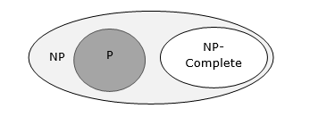
文章目录**P vs NP****0 PNP基本定义**0.1 Definition of NP-Completeness0.2 NP-Complete Problems0.3 NP-Hard Problems0.4 TSP is NP-Complete0.5 Proof**1 PNP问题****2 千禧年世纪难题****3 P类和NP类问题特征****4 多项式时间****5 现实中的NP类问题****6 大突破之NPC问题…

窥探react事件
写在前面 本文源于本人在学习react过程中遇到的一个问题;本文内容为本人的一些的理解,如有不对的地方,还请大家指出来。本文是讲react的事件,不是介绍其api,而是猜想一下react合成事件的实现方式 遇到的问题 class Eve…
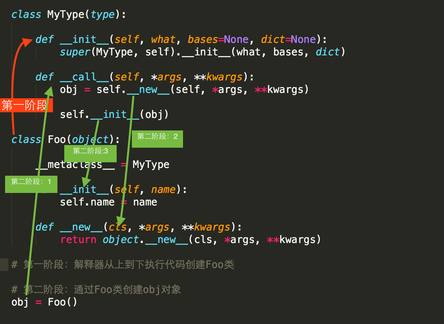
Python内置方法
一、常用的内置方法 1、__new__ 和 __init__: __new__ 构造方法 、__init__初始化函数1、__new__方法是真正的类构造方法,用于产生实例化对象(空属性)。重写__new__方法可以控制对象的产 生过程。也就是说会通过继承object的new方…
【OpenCV 】Sobel 导数/Laplace 算子/Canny 边缘检测
canny边缘检测见OpenCV 【七】————边缘提取算子(图像边缘提取)——canny算法的原理及实现 1 Sobel 导数 1.1.1 原因 上面两节我们已经学习了卷积操作。一个最重要的卷积运算就是导数的计算(或者近似计算). 为什么对图像进行求导是重要的呢? 假设我…
RGB 转 HSV
#include <opencv2/core/core.hpp> #include <opencv2/highgui/highgui.hpp> #include <opencv2/imgproc/imgproc.hpp> #include <iostream> int main() {// 图像源读取及判断cv::Mat srcImage cv::imread("22.jpg");if (!srcImage.data) …
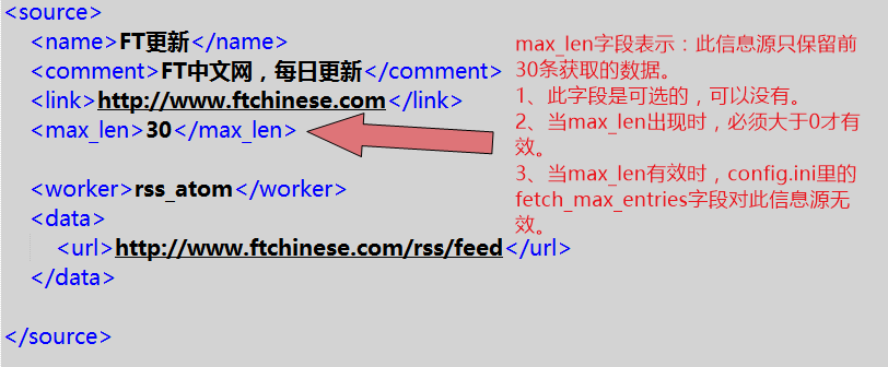
2017.1.9版给信息源新增:max_len、max_db字段
2017.1.8a版程序给信息源增加max_len、max_db字段,分别用于控制:获取条数、数据库保留条数。 max_len的说明见此图: max_db的说明见此图: 当max_len和max_db的设置不合理时(比如max_len大于max_db,会导致反…
索引使用的几个原则
索引的使用尽量满足以下几个原则: 全值匹配最左前缀不在索引列上做任何操作(包括但不限于,计算,函数,类型转换),会导致对应列索引失效。不适用索引中范围条件右边的列尽量使用覆盖索引使用不等于或者not in 的时候回变…

【OpenCV 】Remapping 重映射
目录 1.1目标 1.2 理论 1.3 代码 1.4 运行结果 1.1目标 展示如何使用OpenCV函数 remap 来实现简单重映射. 1.2 理论 把一个图像中一个位置的像素放置到另一个图片指定位置的过程. 为了完成映射过程, 有必要获得一些插值为非整数像素坐标,因为源图像与目标图像的像素坐标…
C# GUID的使用
GUID(全局统一标识符)是指在一台机器上生成的数字,它保证对在同一时空中的所有机器都是唯一的。通常平台会提供生成GUID的API。生成算法很有意思,用到了以太网卡地址、纳秒级时间、芯片ID码和许多可能的数字。GUID的唯一缺陷在于生…
文件名有规则情况读取
#include <iostream> #include <stdio.h> #include <stdlib.h> #include <opencv2/highgui/highgui.hpp> #include <opencv2/imgproc/imgproc.hpp> using namespace cv; using namespace std; int main() {// 定义相关参数const int num 4;char…

编写自己的SpringBoot-starter
2019独角兽企业重金招聘Python工程师标准>>> 前言 原理 首先说说原理,我们知道使用一个公用的starter的时候,只需要将相应的依赖添加的Maven的配置文件当中即可,免去了自己需要引用很多依赖类,并且SpringBoot会自动进行…
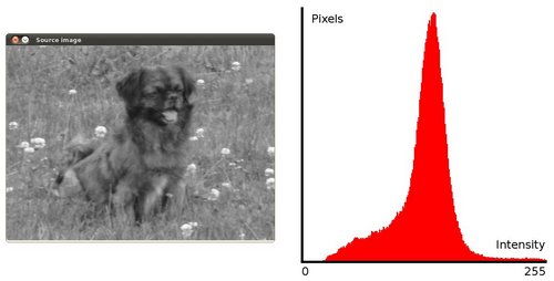
【OpenCV 】直方图均衡化,直方图计算,直方图对比
目录 1.直方图均衡化 1.1 原理 1.2 直方图均衡化 1.3 直方图均衡化原理 1.4 代码实例 1.5 运行效果 2. 直方图计算 2.1 目标 2.2 直方图 2.3 代码实例 2.4 运行结果 3 直方图对比 3.1 目标 3.2 原理 3.3 代码 3.4 运行结果 1.直方图均衡化 什么是图像的直方图和…

c语言实现线性结构(数组与链表)
由于这两天看了数据结构,所以又把大学所学的c语言和指针"挂"起来了。本人菜鸟一枚请多多指教。下面是我这两天学习的成果(数组和链表的实现,用的是c语言哦!哈哈)。(一)数组的实现和操…
OTSU 二值化的实现
#include <stdio.h> #include <string> #include "opencv2/highgui/highgui.hpp" #include "opencv2/opencv.hpp" using namespace std; using namespace cv; // 大均法函数实现 int OTSU(cv::Mat srcImage) {int nCols srcImage.cols;int nR…

vivo7.0系统机器(亲测有效)激活Xposed框架的教程
对于喜欢搞机的机友来说,常常会使用到Xposed框架和种种功能牛逼的模块,对于5.0以下的系统版本,只要手机能获得Root权限,安装和激活Xposed框架是异常轻松的,但随着系统版本的升级,5.0以后的系统,…

【OpenCV 】反向投影
目录 1 目标 2原理:什么是反向投影? 3 代码实现 4 实现结果 1 目标 什么是反向投影,它可以实现什么功能? 如何使用OpenCV函数 calcBackProject 计算反向投影? 如何使用OpenCV函数 mixChannels 组合图像的不同通道…
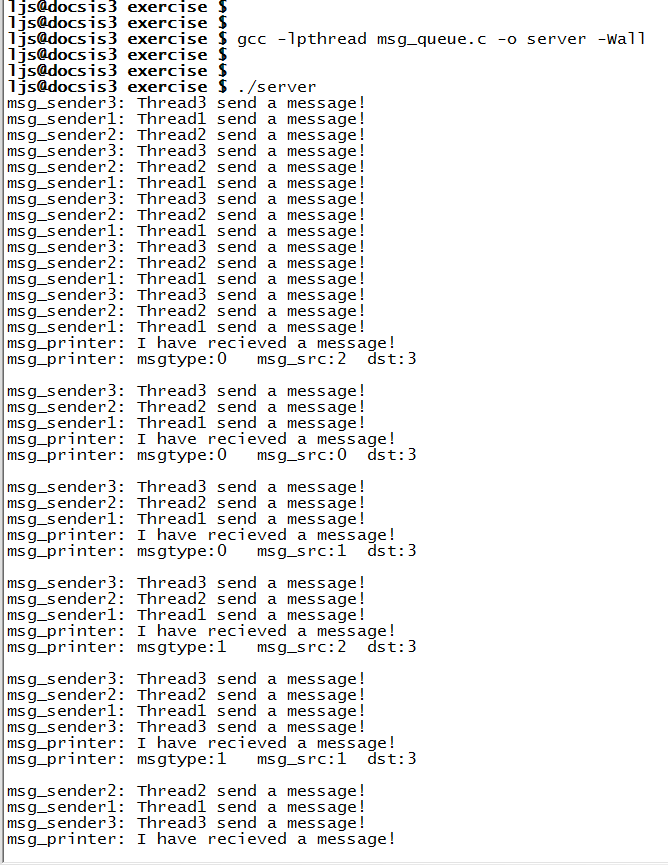
Linux编程之自定义消息队列
我这里要讲的并不是IPC中的消息队列,我要讲的是在进程内部实现自定义的消息队列,让各个线程的消息来推动整个进程的运动。进程间的消息队列用于进程与进程之间的通信,而我将要实现的进程内的消息队列是用于有序妥当处理来自于各个线程请求&am…
threshold 二值化的实现
#include "opencv2/imgproc/imgproc.hpp" #include "opencv2/highgui/highgui.hpp" int main( ) {// 读取源图像及判断cv::Mat srcImage cv::imread("..\\images\\hand1.jpg");if( !srcImage.data ) return 1;// 转化为灰度图像cv::Mat srcGray…
如何定时备份数据库并上传七牛云
前言: 这篇文章主要记录自己在备份数据库文件中踩的坑和解决办法。 服务器数据库备份文件之后上传到七牛云 备份数据库文件在服务器根目录下 创建 /backup/qiniu/.backup.sh #!/bin/bash# vuemall 数据库名称 # blog_runner vuemall 的管理用户# admin vuem…

【OpenCV 】计算物体的凸包/创建包围轮廓的矩形和圆形边界框/createTrackbar添加滑动条/
目录 topic 1:模板匹配 topic 2:图像中寻找轮廓 topic 3:计算物体的凸包 topic 4:轮廓创建可倾斜的边界框和椭圆 topic 5:轮廓矩 topic 6:为程序界面添加滑动条 3.1 目标 3.2 代码实例1 3.3 代码实例2 3.4 实例3运行结果 3.5 运行结果 topic 1:模板匹配 topic 2:图…
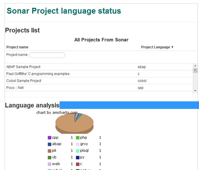
开源:Angularjs示例--Sonar中项目使用语言分布图
在博客中介绍google的Angularjs 客户端PM模式框架很久了,今天发布一个关于AngularJs使用是简单示例SonarLanguage(示例位于Github:https://github.com/greengerong/SonarLanguage)。本项目只是一个全为客户端的示例项目。项目的初始是我想看看在公司的项…
adaptiveThreshold 阈值化的实现
#include "opencv2/imgproc/imgproc.hpp" #include "opencv2/highgui/highgui.hpp" int main( ) {// 图像读取及判断cv::Mat srcImage cv::imread("..\\images\\hand1.jpg");if( !srcImage.data ) return 1;// 灰度转换cv::Mat srcGray;cv::cvt…
hashMap传入参数,table长度为多少
前言 我的所有文章同步更新与Github--Java-Notes,想了解JVM,HashMap源码分析,spring相关,剑指offer题解(Java版),可以点个star。可以看我的github主页,每天都在更新哟。 邀请您跟我一同完成 rep…
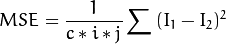
【OpenCV】图像/视频相似度测量PSNR( Peak signal-to-noise ratio) and SSIM,视频/图片转换
目录 1 目标 2 原理 2.1 图像比较 - PSNR and SSIM 3 代码 3.1如何读取一个视频流(摄像头或者视频文件)? 3 运行效果 视频/图片转换: 如何用OpenCV创建一个视频文件用OpenCV能创建什么样的视频文件如何释放视频文件当中的某个颜色通道…
struts2提交list
2019独角兽企业重金招聘Python工程师标准>>> Action: private List<User> users; jsp: <input type"text" name"users[0].name" value"aaa" /> <input type"text" name"users[1].name" value&q…
双阈值法的实现
#include "opencv2/imgproc/imgproc.hpp" #include "opencv2/highgui/highgui.hpp" int main( ) {// 图像读取及判断cv::Mat srcImage cv::imread("..\\images\\hand1.jpg");if( !srcImage.data ) return 1;// 灰度转换cv::Mat srcGray;cv::cvt…
设计模式 小记
观察者模式 1.被观察者是单例模式。 生成这模式 1.Director中对于Builder的引用不一定是Strong,根据情况也有可能是Copy。 2.Director 聚合 Builder, 所以Builder本身可以单独拿出来使用。 转载于:https://juejin.im/post/5ca8c24df265da3094116c18