通俗易懂!使用Excel和TF实现Transformer

作者 | 石晓文
转载自小小挖掘机(ID:wAIsjwj)
本文旨在通过最通俗易懂的过程来详解Transformer的每个步骤!
假设我们在做一个从中文翻译到英文的过程,我们的词表很简单如下:
中文词表:[机、器、学、习] 英文词表[deep、machine、learning、chinese]
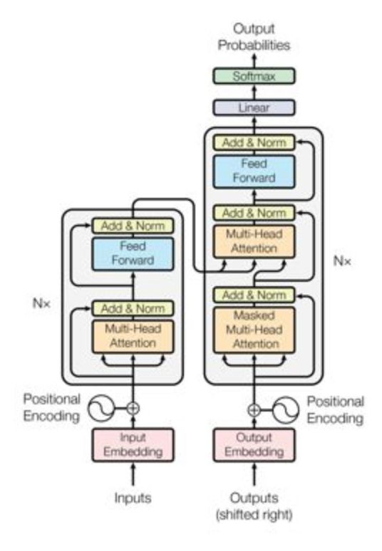
先来看一下Transformer的整个过程:
接下来,我们将按顺序来讲解Transformer的过程,并配有配套的excel计算过程和tensorflow代码。
先说明一下,本文的tensorflow代码中使用两条训练数据(因为实际场景中输入都是batch的),但excel计算只以第一条数据的处理过程为例。
1、Encoder输入
Encoder输入过程如下图所示:

首先输入数据会转换为对应的embedding,然后会加上位置偏置,得到最终的输入。
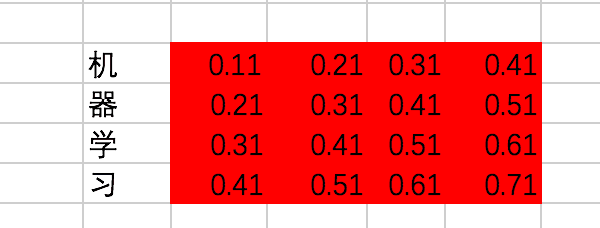
这里,为了结果的准确计算,我们使用常量来代表embedding,假设中文词表对应的embedding值分别是:
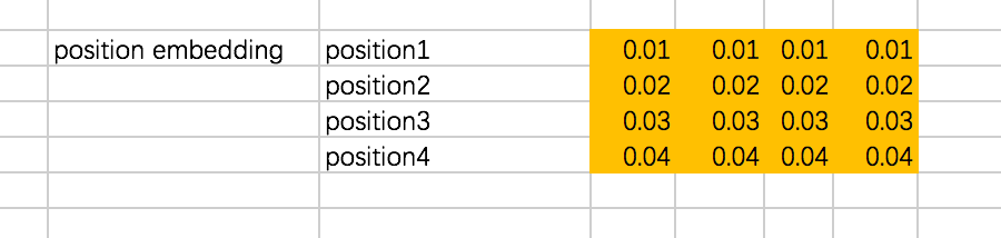
位置偏置position embedding使用下面的式子计算得出,注意这里位置偏置是包含两个维度的,不仅仅是encoder的第几个输入,同时embedding中的每一个维度都会加入位置偏置信息:
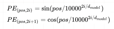
不过为了计算方便,我们仍然使用固定值代替:
假设我们有两条训练数据(Excel大都只以第一条数据为例):
[机、器、学、习] -> [ machine、learning]
[学、习、机、器] -> [learning、machine]
encoder的输入在转换成id后变为[[0,1,2,3],[2,3,0,1]]。
接下来,通过查找中文的embedding表,转换为embedding为:
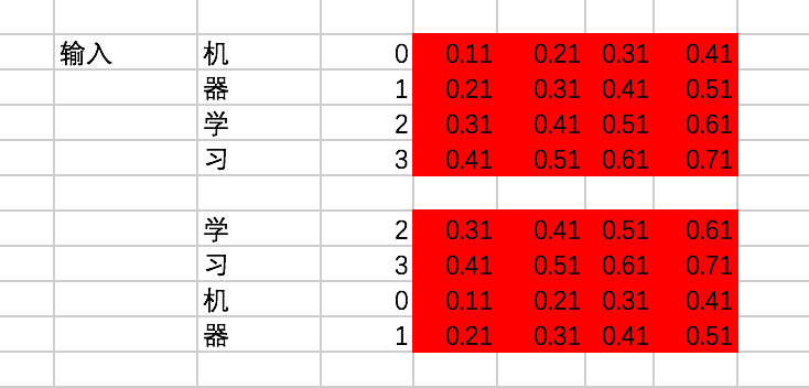
对输入加入位置偏置,注意这里是两个向量的对位相加:
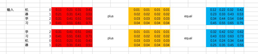
上面的过程是这样的,接下来咱们用代码来表示一下:
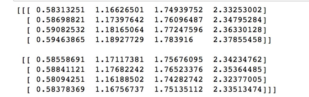
import tensorflow as tfchinese_embedding = tf.constant([[0.11,0.21,0.31,0.41], [0.21,0.31,0.41,0.51], [0.31,0.41,0.51,0.61], [0.41,0.51,0.61,0.71]],dtype=tf.float32)english_embedding = tf.constant([[0.51,0.61,0.71,0.81], [0.52,0.62,0.72,0.82], [0.53,0.63,0.73,0.83], [0.54,0.64,0.74,0.84]],dtype=tf.float32)position_encoding = tf.constant([[0.01,0.01,0.01,0.01], [0.02,0.02,0.02,0.02], [0.03,0.03,0.03,0.03], [0.04,0.04,0.04,0.04]],dtype=tf.float32)encoder_input = tf.constant([[0,1,2,3],[2,3,0,1]],dtype=tf.int32)with tf.variable_scope("encoder_input"): encoder_embedding_input = tf.nn.embedding_lookup(chinese_embedding,encoder_input) encoder_embedding_input = encoder_embedding_input + position_encodingwith tf.Session() as sess: sess.run(tf.global_variables_initializer()) print(sess.run([encoder_embedding_input]))结果为:
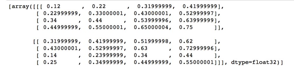
跟刚才的结果保持一致。
2、Encoder Block
一个Encoder的Block过程如下:
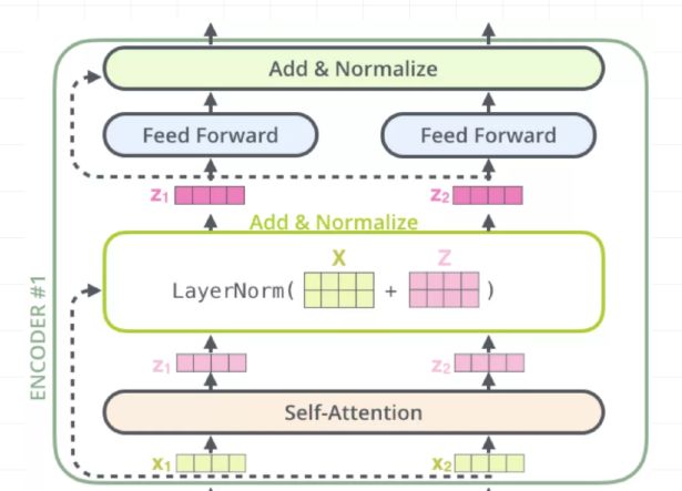
分为4步,分别是multi-head self attention、Add & Normalize、Feed Forward Network、Add & Normalize。
咱们主要来讲multi-head self attention。在讲multi-head self attention的时候,先讲讲Scaled Dot-Product Attention,我有时候也称为single-head self attention。
2.1 Attention机制简单回顾
Attention其实就是计算一种相关程度,看下面的例子:
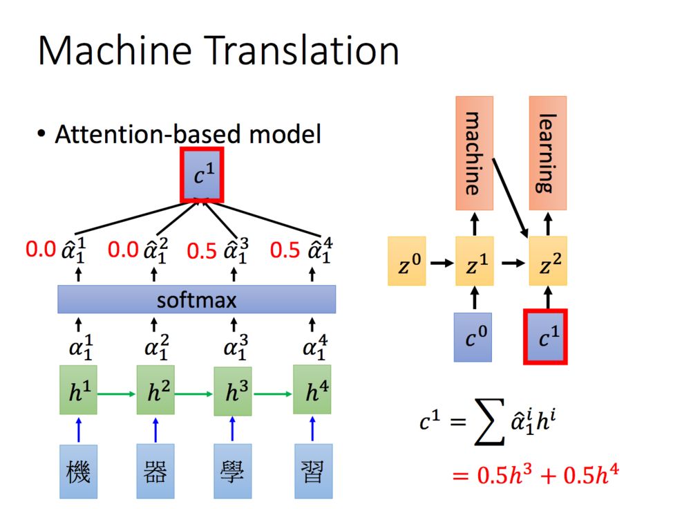
Attention通常可以进行如下描述,表示为将query(Q)和key-value pairs映射到输出上,其中query、每个key、每个value都是向量,输出是V中所有values的加权,其中权重是由Query和每个key计算出来的,计算方法分为三步:
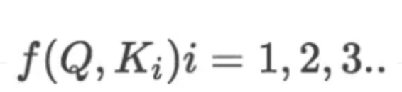
1)计算比较Q和K的相似度,用f来表示:
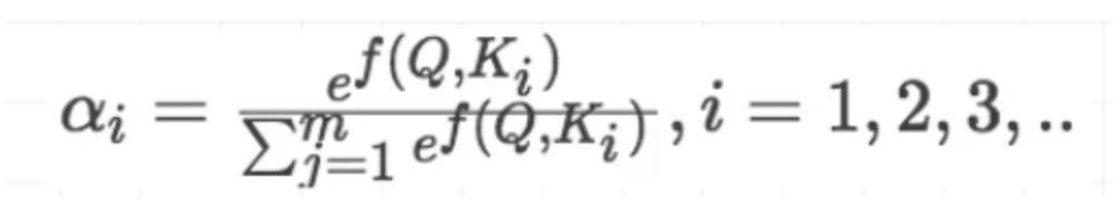
2)将得到的相似度进行softmax归一化:
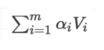
3)针对计算出来的权重,对所有的values进行加权求和,得到Attention向量:
计算相似度的方法有以下4种:
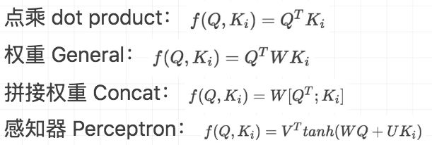
在本文中,我们计算相似度的方式是第一种。
2.2 Scaled Dot-Product Attention
咱们先说说Q、K、V。比如我们想要计算上图中machine和机、器、学、习四个字的attention,并加权得到一个输出,那么Query由machine对应的embedding计算得到,K和V分别由机、器、学、习四个字对应的embedding得到。
在encoder的self-attention中,由于是计算自身和自身的相似度,所以Q、K、V都是由输入的embedding得到的,不过我们还是加以区分。
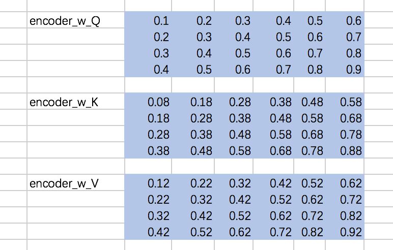
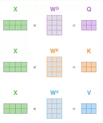
这里, Q、K、V分别通过一层全连接神经网络得到,同样,我们把对应的参数矩阵都写作常量。
接下来,我们得到的到Q、K、V,我们以第一条输入为例:
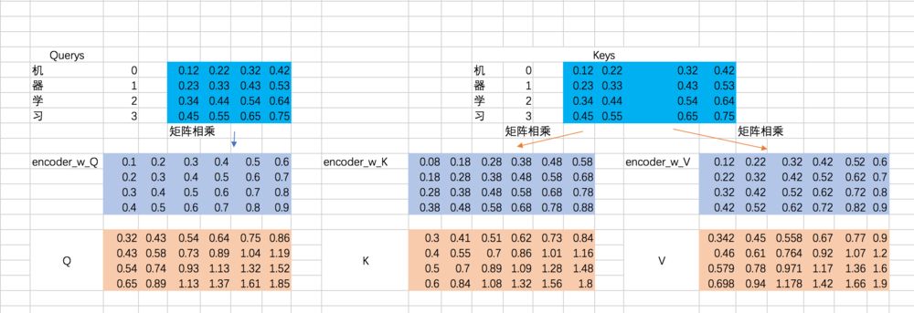
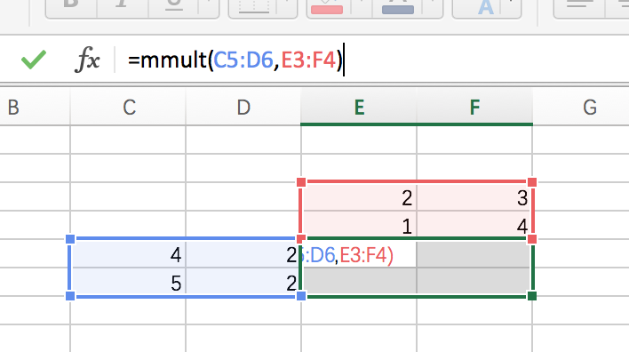
既然是一层全连接嘛,所以相当于一次矩阵相乘,excel里面的矩阵相乘如下:
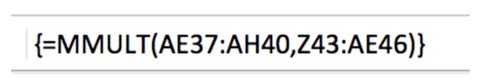
在Mac中,一定要先选中对应大小的区域,输入公式,然后使用command + shift + enter才能一次性得到全部的输出,如下图:
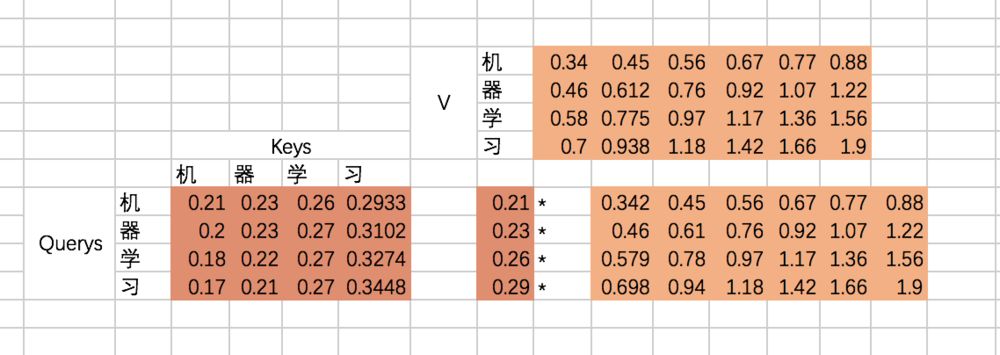
接下来,我们要去计算Q和K的相关性大小了,这里使用内积的方式,相当于QKT:
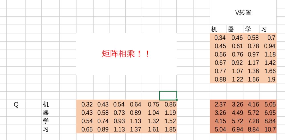
(上图应该是K,不影响整个过程理解)同样,excel中的转置,也要选择相应的区域后,使用transpose函数,然后按住command + shift + enter一次性得到全部输出。
我们来看看结果代表什么含义:
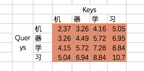
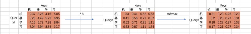
也就是说,机和机自身的相关性是2.37(未进行归一化处理),机和器的相关性是3.26,依次类推。我们可以称上述的结果为raw attention map。对于raw attention map,我们需要进行两步处理,首先是除以一个规范化因子,然后进行softmax操作,这里的规范化因子选择除以8,然后每行进行一个softmax归一化操作(按行做归一化是因为attention的初衷是计算每个Query和所有的Keys之间的相关性):
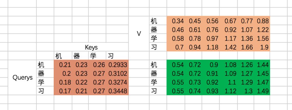
最后就是得到每个输入embedding 对应的输出embedding,也就是基于attention map对V进行加权求和,以“机”这个输入为例,最后的输出应该是V对应的四个向量的加权求和:
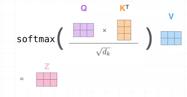
如果用矩阵表示,那么最终的结果是规范化后的attention map和V矩阵相乘,因此最终结果是:
至此,我们的Scaled Dot-Product Attention的过程就全部计算完了,来看看代码吧:
with tf.variable_scope("encoder_scaled_dot_product_attention"): encoder_Q = tf.matmul(tf.reshape(encoder_embedding_input,(-1,tf.shape(encoder_embedding_input)[2])),w_Q) encoder_K = tf.matmul(tf.reshape(encoder_embedding_input,(-1,tf.shape(encoder_embedding_input)[2])),w_K) encoder_V = tf.matmul(tf.reshape(encoder_embedding_input,(-1,tf.shape(encoder_embedding_input)[2])),w_V) encoder_Q = tf.reshape(encoder_Q,(tf.shape(encoder_embedding_input)[0],tf.shape(encoder_embedding_input)[1],-1)) encoder_K = tf.reshape(encoder_K,(tf.shape(encoder_embedding_input)[0],tf.shape(encoder_embedding_input)[1],-1)) encoder_V = tf.reshape(encoder_V,(tf.shape(encoder_embedding_input)[0],tf.shape(encoder_embedding_input)[1],-1)) attention_map = tf.matmul(encoder_Q,tf.transpose(encoder_K,[0,2,1])) attention_map = attention_map / 8 attention_map = tf.nn.softmax(attention_map)with tf.Session() as sess: sess.run(tf.global_variables_initializer()) print(sess.run(attention_map)) print(sess.run(encoder_first_sa_output))第一条数据的attention map为:
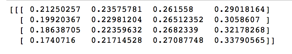
第一条数据的输出为:
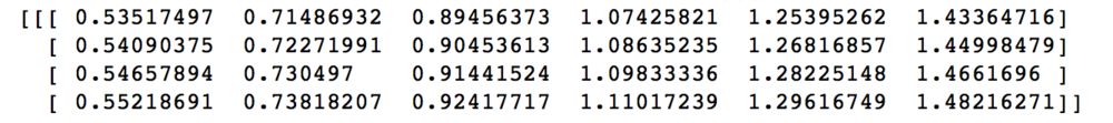
可以看到,跟我们通过excel计算得到的输出也是保持一致的。
咱们再通过图片来回顾下Scaled Dot-Product Attention的过程:
2.3 multi-head self attention
Multi-Head Attention就是把Scaled Dot-Product Attention的过程做H次,然后把输出Z合起来。
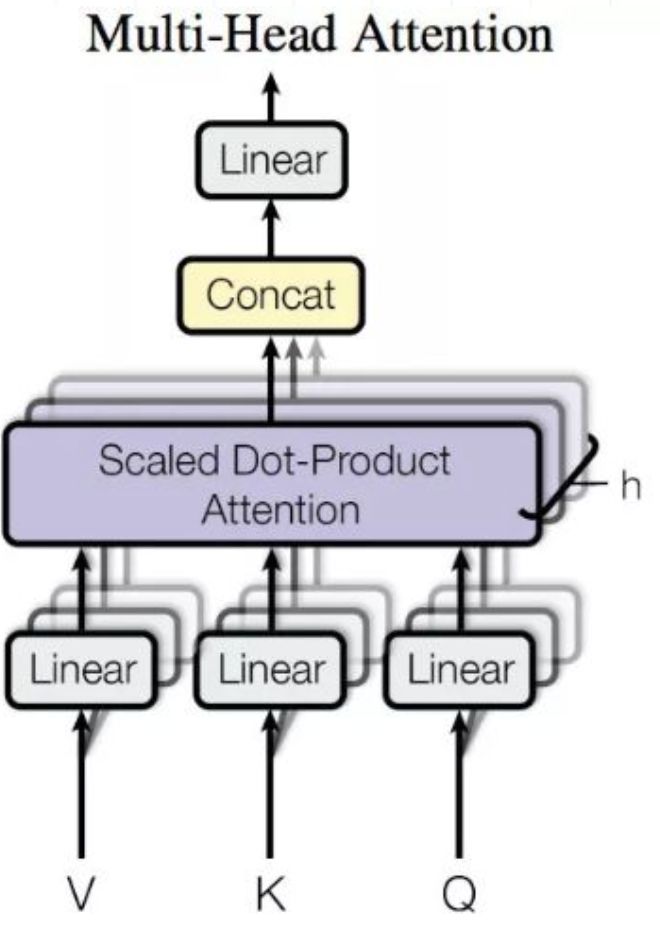
整个过程图示如下:
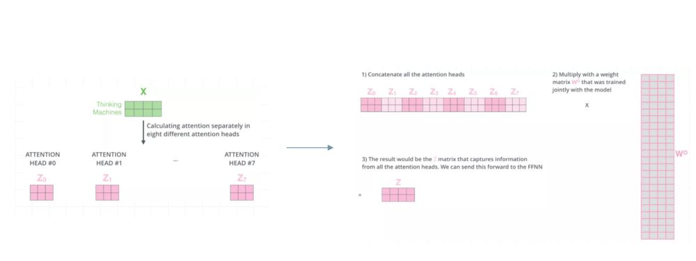
这里,我们还是先用excel的过程计算一遍。假设我们刚才计算得到的Q、K、V从中间切分,分别作为两个Head的输入:
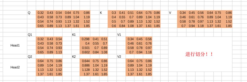
重复上面的Scaled Dot-Product Attention过程,我们分别得到两个Head的输出:
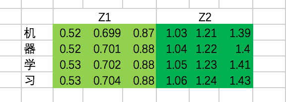
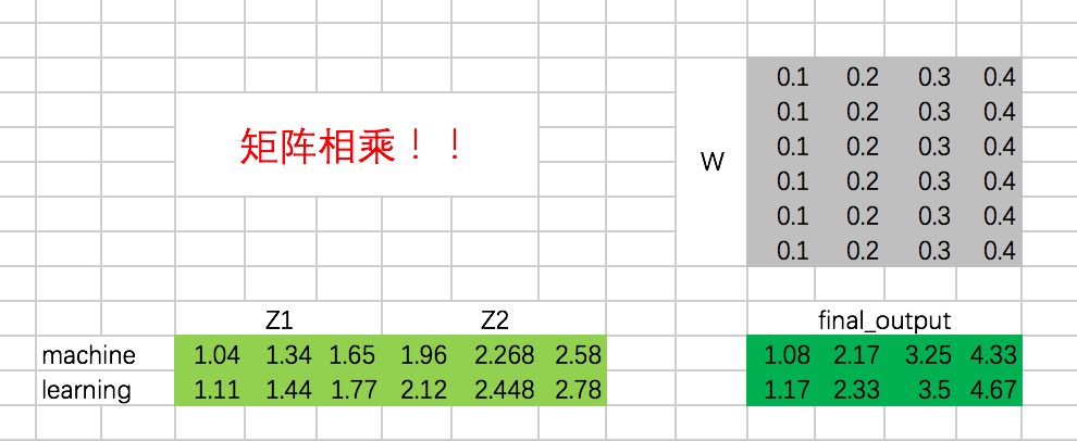
接下来,我们需要通过一个权重矩阵,来得到最终输出。
为了我们能够进行后面的Add的操作,我们需要把输出的长度和输入保持一致,即每个单词得到的输出embedding长度保持为4。
同样,我们这里把转换矩阵W设置为常数:
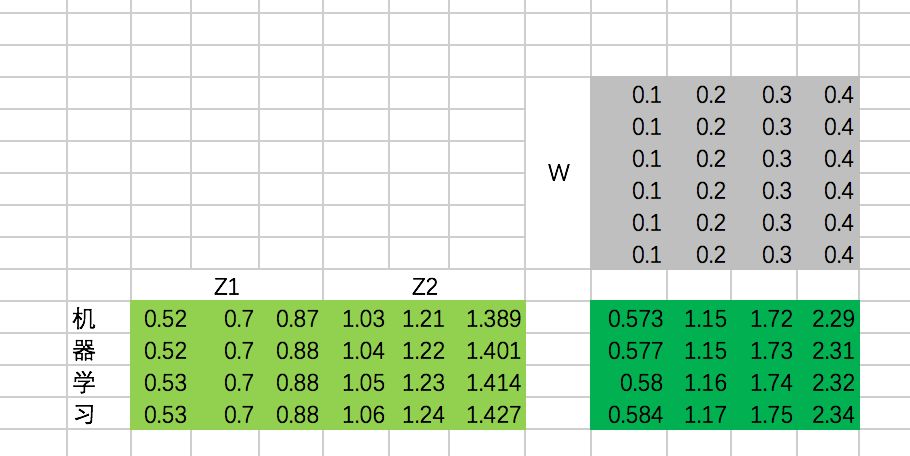
最终,每个单词在经过multi-head attention之后,得到的输出为:
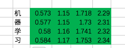
好了,开始写代码吧:
w_Z = tf.constant([[0.1,0.2,0.3,0.4], [0.1,0.2,0.3,0.4], [0.1,0.2,0.3,0.4], [0.1,0.2,0.3,0.4], [0.1,0.2,0.3,0.4], [0.1,0.2,0.3,0.4]],dtype=tf.float32)with tf.variable_scope("encoder_input"): encoder_embedding_input = tf.nn.embedding_lookup(chinese_embedding,encoder_input) encoder_embedding_input = encoder_embedding_input + position_encodingwith tf.variable_scope("encoder_multi_head_product_attention"): encoder_Q = tf.matmul(tf.reshape(encoder_embedding_input,(-1,tf.shape(encoder_embedding_input)[2])),w_Q) encoder_K = tf.matmul(tf.reshape(encoder_embedding_input,(-1,tf.shape(encoder_embedding_input)[2])),w_K) encoder_V = tf.matmul(tf.reshape(encoder_embedding_input,(-1,tf.shape(encoder_embedding_input)[2])),w_V) encoder_Q = tf.reshape(encoder_Q,(tf.shape(encoder_embedding_input)[0],tf.shape(encoder_embedding_input)[1],-1)) encoder_K = tf.reshape(encoder_K,(tf.shape(encoder_embedding_input)[0],tf.shape(encoder_embedding_input)[1],-1)) encoder_V = tf.reshape(encoder_V,(tf.shape(encoder_embedding_input)[0],tf.shape(encoder_embedding_input)[1],-1)) encoder_Q_split = tf.split(encoder_Q,2,axis=2) encoder_K_split = tf.split(encoder_K,2,axis=2) encoder_V_split = tf.split(encoder_V,2,axis=2) encoder_Q_concat = tf.concat(encoder_Q_split,axis=0) encoder_K_concat = tf.concat(encoder_K_split,axis=0) encoder_V_concat = tf.concat(encoder_V_split,axis=0) attention_map = tf.matmul(encoder_Q_concat,tf.transpose(encoder_K_concat,[0,2,1])) attention_map = attention_map / 8 attention_map = tf.nn.softmax(attention_map) weightedSumV = tf.matmul(attention_map,encoder_V_concat) outputs_z = tf.concat(tf.split(weightedSumV,2,axis=0),axis=2) outputs = tf.matmul(tf.reshape(outputs_z,(-1,tf.shape(outputs_z)[2])),w_Z) outputs = tf.reshape(outputs,(tf.shape(encoder_embedding_input)[0],tf.shape(encoder_embedding_input)[1],-1)) import numpy as npwith tf.Session() as sess:# print(sess.run(encoder_Q))# print(sess.run(encoder_Q_split)) #print(sess.run(weightedSumV)) #print(sess.run(outputs_z)) print(sess.run(outputs))结果的输出为:
这里的结果其实和excel是一致的,细小的差异源于excel在复制粘贴过程中,小数点的精度有所损失。
这里我们主要来看下两个函数,分别是split和concat,理解这两个函数的过程对明白上述代码至关重要。
split函数主要有三个参数,第一个是要split的tensor,第二个是分割成几个tensor,第三个是在哪一维进行切分。也就是说, encoder_Q_split = tf.split(encoder_Q,2,axis=2),执行这段代码的话,encoder_Q这个tensor会按照axis=2切分成两个同样大的tensor,这两个tensor的axis=0和axis=1维度的长度是不变的,但axis=2的长度变为了一半,我们在后面通过图示的方式来解释。
从代码可以看到,共有两次split和concat的过程,第一次是将Q、K、V切分为不同的Head:
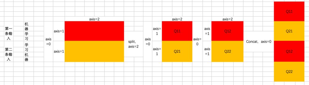
也就是说,原先每条数据的所对应的各Head的Q并非相连的,而是交替出现的,即 [Head1-Q11,Head1-Q21,Head2-Q12,Head2-Q22]
第二次是最后计算完每个Head的输出Z之后,通过split和concat进行还原,过程如下:
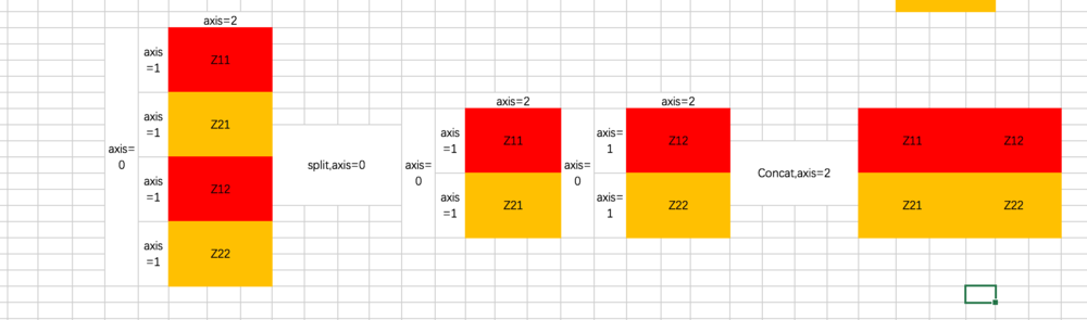
上面的图示咱们将三维矩阵操作抽象成了二维,我加入了axis的说明帮助你理解。如果不懂的话,单步执行下代码就会懂啦。
2.4 Add & Normalize & FFN
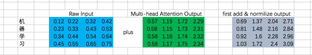
后面的过程其实很多简单了,我们继续用excel来表示一下,这里,我们忽略BN的操作(大家可以加上,这里主要是比较麻烦哈哈)
第一次Add & Normalize
接下来是一个FFN,我们仍然假设是固定的参数,那么output是:
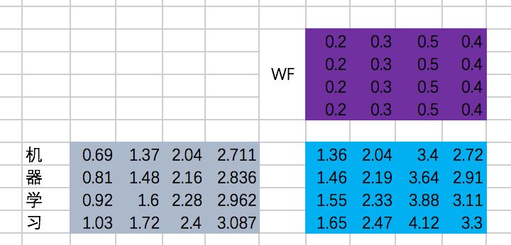
第二次Add & Normalize
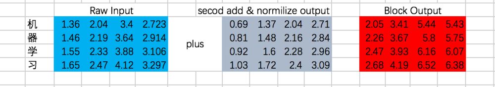
我们终于在经过一个Encoder的Block后得到了每个输入对应的输出,分别为:
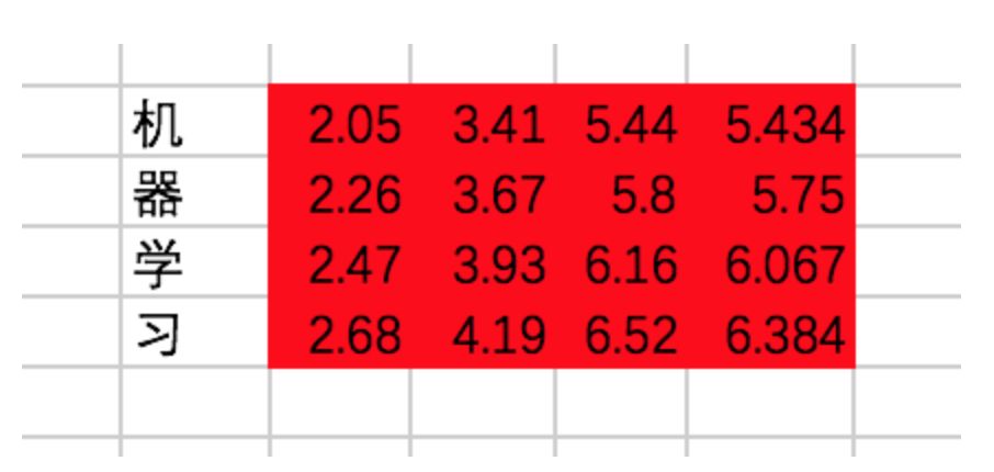
让我们把这段代码补充上去吧:
with tf.variable_scope("encoder_block"): encoder_Q = tf.matmul(tf.reshape(encoder_embedding_input,(-1,tf.shape(encoder_embedding_input)[2])),w_Q) encoder_K = tf.matmul(tf.reshape(encoder_embedding_input,(-1,tf.shape(encoder_embedding_input)[2])),w_K) encoder_V = tf.matmul(tf.reshape(encoder_embedding_input,(-1,tf.shape(encoder_embedding_input)[2])),w_V) encoder_Q = tf.reshape(encoder_Q,(tf.shape(encoder_embedding_input)[0],tf.shape(encoder_embedding_input)[1],-1)) encoder_K = tf.reshape(encoder_K,(tf.shape(encoder_embedding_input)[0],tf.shape(encoder_embedding_input)[1],-1)) encoder_V = tf.reshape(encoder_V,(tf.shape(encoder_embedding_input)[0],tf.shape(encoder_embedding_input)[1],-1)) encoder_Q_split = tf.split(encoder_Q,2,axis=2) encoder_K_split = tf.split(encoder_K,2,axis=2) encoder_V_split = tf.split(encoder_V,2,axis=2) encoder_Q_concat = tf.concat(encoder_Q_split,axis=0) encoder_K_concat = tf.concat(encoder_K_split,axis=0) encoder_V_concat = tf.concat(encoder_V_split,axis=0) attention_map = tf.matmul(encoder_Q_concat,tf.transpose(encoder_K_concat,[0,2,1])) attention_map = attention_map / 8 attention_map = tf.nn.softmax(attention_map) weightedSumV = tf.matmul(attention_map,encoder_V_concat) outputs_z = tf.concat(tf.split(weightedSumV,2,axis=0),axis=2) sa_outputs = tf.matmul(tf.reshape(outputs_z,(-1,tf.shape(outputs_z)[2])),w_Z) sa_outputs = tf.reshape(sa_outputs,(tf.shape(encoder_embedding_input)[0],tf.shape(encoder_embedding_input)[1],-1)) sa_outputs = sa_outputs + encoder_embedding_input # todo :add BN W_f = tf.constant([[0.2,0.3,0.5,0.4], [0.2,0.3,0.5,0.4], [0.2,0.3,0.5,0.4], [0.2,0.3,0.5,0.4]]) ffn_outputs = tf.matmul(tf.reshape(sa_outputs,(-1,tf.shape(sa_outputs)[2])),W_f) ffn_outputs = tf.reshape(ffn_outputs,(tf.shape(sa_outputs)[0],tf.shape(sa_outputs)[1],-1)) encoder_outputs = ffn_outputs + sa_outputs # todo :add BNimport numpy as npwith tf.Session() as sess:# print(sess.run(encoder_Q))# print(sess.run(encoder_Q_split)) #print(sess.run(weightedSumV)) #print(sess.run(outputs_z)) #print(sess.run(sa_outputs)) #print(sess.run(ffn_outputs)) print(sess.run(encoder_outputs))输出为:
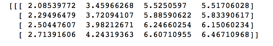
与excel计算结果基本一致。
当然,encoder的各层是可以堆叠的,但我们这里只以单层的为例,重点是理解整个过程。
3、Decoder Block
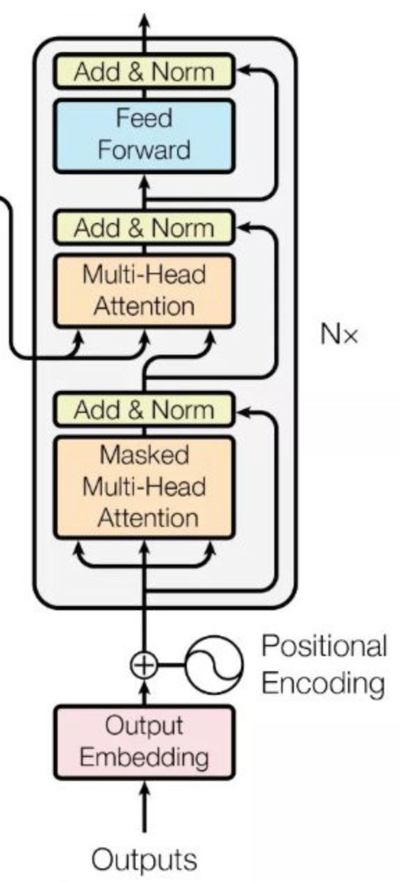
一个Decoder的Block过程如下:
相比Encoder,这里的过程分为6步,分别是 masked multi-head self attention、Add & Normalize、encoder-decoder attention、Add & Normalize、Feed Forward Network、Add & Normalize。
咱们还是重点来讲masked multi-head self attention和encoder-decoder attention。
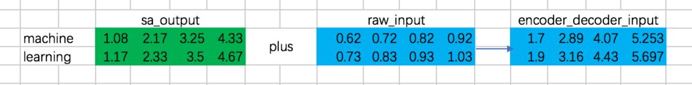
3.1 Decoder输入
这里,在excel中,咱们还是以第一条输入为例,来展示整个过程:
[机、器、学、习] -> [ machine、learning]
因此,Decoder阶段的输入是:
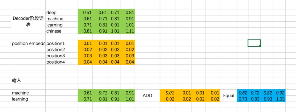
对应的代码如下:
english_embedding = tf.constant([[0.51,0.61,0.71,0.81], [0.61,0.71,0.81,0.91], [0.71,0.81,0.91,1.01], [0.81,0.91,1.01,1.11]],dtype=tf.float32)position_encoding = tf.constant([[0.01,0.01,0.01,0.01], [0.02,0.02,0.02,0.02], [0.03,0.03,0.03,0.03], [0.04,0.04,0.04,0.04]],dtype=tf.float32)decoder_input = tf.constant([[1,2],[2,1]],dtype=tf.int32)with tf.variable_scope("decoder_input"): decoder_embedding_input = tf.nn.embedding_lookup(english_embedding,decoder_input) decoder_embedding_input = decoder_embedding_input + position_encoding[0:tf.shape(decoder_embedding_input)[1]]3.2 masked multi-head self attention
这个过程和multi-head self attention基本一致,只不过对于decoder来说,得到每个阶段的输出时,我们是看不到后面的信息的。举个例子,我们的第一条输入是:[机、器、学、习] -> [ machine、learning] ,decoder阶段两次的输入分别是machine和learning,在输入machine时,我们是看不到learning的信息的,因此在计算attention的权重的时候,machine和learning的权重是没有的。我们还是先通过excel来演示一下,再通过代码来理解:
计算Attention的权重矩阵是:
仍然以两个Head为例,计算Q、K、V:
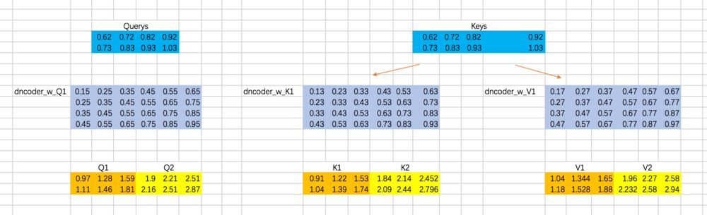
分别计算两个Head的attention map
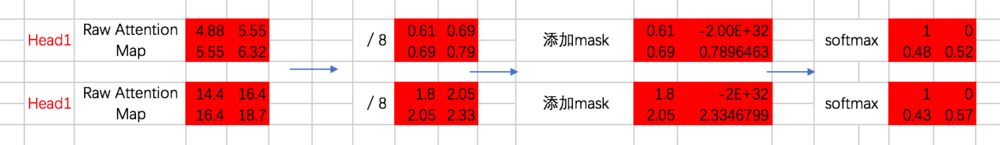
咱们先来实现这部分的代码,masked attention map的计算过程:
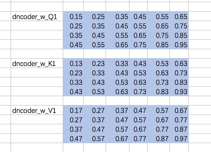
先定义下权重矩阵,同encoder一样,定义成常数:
w_Q_decoder_sa = tf.constant([[0.15,0.25,0.35,0.45,0.55,0.65], [0.25,0.35,0.45,0.55,0.65,0.75], [0.35,0.45,0.55,0.65,0.75,0.85], [0.45,0.55,0.65,0.75,0.85,0.95]],dtype=tf.float32)w_K_decoder_sa = tf.constant([[0.13,0.23,0.33,0.43,0.53,0.63], [0.23,0.33,0.43,0.53,0.63,0.73], [0.33,0.43,0.53,0.63,0.73,0.83], [0.43,0.53,0.63,0.73,0.83,0.93]],dtype=tf.float32)w_V_decoder_sa = tf.constant([[0.17,0.27,0.37,0.47,0.57,0.67], [0.27,0.37,0.47,0.57,0.67,0.77], [0.37,0.47,0.57,0.67,0.77,0.87], [0.47,0.57,0.67,0.77,0.87,0.97]],dtype=tf.float32)随后,计算添加mask之前的attention map:
with tf.variable_scope("decoder_sa_block"): decoder_Q = tf.matmul(tf.reshape(decoder_embedding_input,(-1,tf.shape(decoder_embedding_input)[2])),w_Q_decoder_sa) decoder_K = tf.matmul(tf.reshape(decoder_embedding_input,(-1,tf.shape(decoder_embedding_input)[2])),w_K_decoder_sa) decoder_V = tf.matmul(tf.reshape(decoder_embedding_input,(-1,tf.shape(decoder_embedding_input)[2])),w_V_decoder_sa) decoder_Q = tf.reshape(decoder_Q,(tf.shape(decoder_embedding_input)[0],tf.shape(decoder_embedding_input)[1],-1)) decoder_K = tf.reshape(decoder_K,(tf.shape(decoder_embedding_input)[0],tf.shape(decoder_embedding_input)[1],-1)) decoder_V = tf.reshape(decoder_V,(tf.shape(decoder_embedding_input)[0],tf.shape(decoder_embedding_input)[1],-1)) decoder_Q_split = tf.split(decoder_Q,2,axis=2) decoder_K_split = tf.split(decoder_K,2,axis=2) decoder_V_split = tf.split(decoder_V,2,axis=2) decoder_Q_concat = tf.concat(decoder_Q_split,axis=0) decoder_K_concat = tf.concat(decoder_K_split,axis=0) decoder_V_concat = tf.concat(decoder_V_split,axis=0) decoder_sa_attention_map_raw = tf.matmul(decoder_Q_concat,tf.transpose(decoder_K_concat,[0,2,1])) decoder_sa_attention_map = decoder_sa_attention_map_raw / 8随后,对attention map添加mask:
diag_vals = tf.ones_like(decoder_sa_attention_map[0,:,:])tril = tf.contrib.linalg.LinearOperatorTriL(diag_vals).to_dense()masks = tf.tile(tf.expand_dims(tril,0),[tf.shape(decoder_sa_attention_map)[0],1,1])paddings = tf.ones_like(masks) * (-2 ** 32 + 1)decoder_sa_attention_map = tf.where(tf.equal(masks,0),paddings,decoder_sa_attention_map)decoder_sa_attention_map = tf.nn.softmax(decoder_sa_attention_map)这里我们首先构造一个全1的矩阵diag_vals,这个矩阵的大小同attention map。随后通过tf.contrib.linalg.LinearOperatorTriL方法把上三角部分变为0,该函数的示意如下:
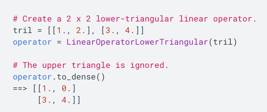
基于这个函数生成的矩阵tril,我们便可以构造对应的mask了。不过需要注意的是,对于我们要加mask的地方,不能赋值为0,而是需要赋值一个很小的数,这里为-2^32 + 1。因为我们后面要做softmax,e^0=1,是一个很大的数啦。
运行上面的代码:
import numpy as npwith tf.Session() as sess: print(sess.run(decoder_sa_attention_map))观察第一条数据对应的结果如下:
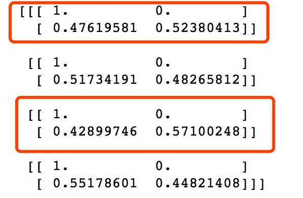
与我们excel计算结果相吻合。
后面的过程我们就不详细介绍了,我们直接给出经过masked multi-head self attention的对应结果:
对应的代码如下:
weightedSumV = tf.matmul(decoder_sa_attention_map,decoder_V_concat) decoder_outputs_z = tf.concat(tf.split(weightedSumV,2,axis=0),axis=2) decoder_sa_outputs = tf.matmul(tf.reshape(decoder_outputs_z,(-1,tf.shape(decoder_outputs_z)[2])),w_Z_decoder_sa) decoder_sa_outputs = tf.reshape(decoder_sa_outputs,(tf.shape(decoder_embedding_input)[0],tf.shape(decoder_embedding_input)[1],-1))with tf.Session() as sess: print(sess.run(decoder_sa_outputs))输出为:

与excel保持一致!
3.3 encoder-decoder attention
在encoder-decoder attention之间,还有一个Add & Normalize的过程,同样,我们忽略 Normalize,只做Add操作:
接下来,就是encoder-decoder了,这里跟multi-head attention相同,但是需要注意的一点是,我们这里想要做的是,计算decoder的每个阶段的输入和encoder阶段所有输出的attention,所以Q的计算通过decoder对应的embedding计算,而K和V通过encoder阶段输出的embedding来计算:
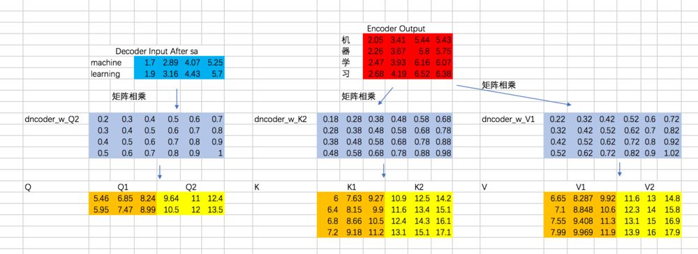
接下来,计算Attention Map,注意,这里attention map的大小为2 * 4的,每一行代表一个decoder的输入,与所有encoder输出之间的attention score。同时,我们不需要添加mask,因为decoder的输入是可以看到所有encoder的输出信息的。得到的attention map结果如下:
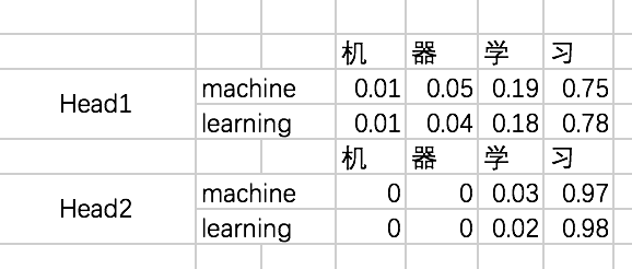
哈哈,这里数是我瞎写的,结果不太好,不过不影响对整个过程的理解。
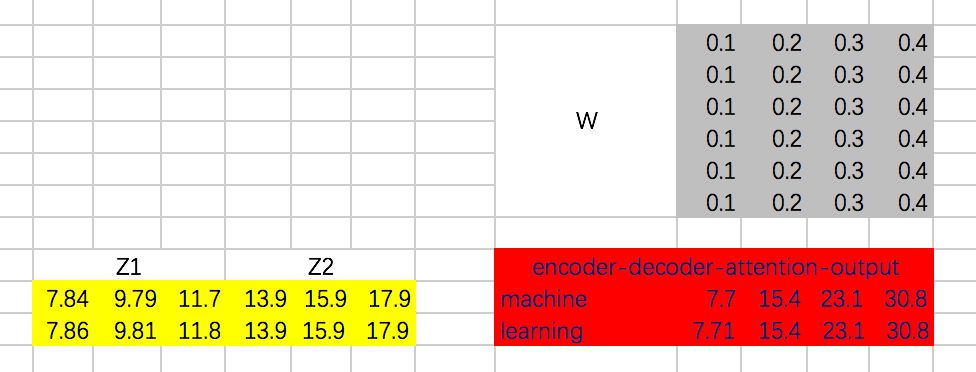
接下来,我们得到整个encoder-decoder阶段的输出为:
接下来,还有Add & Normalize、Feed Forward Network、Add & Normalize过程,咱们这里就省略了。直接上代码吧:
w_Q_decoder_sa2 = tf.constant([[0.2,0.3,0.4,0.5,0.6,0.7], [0.3,0.4,0.5,0.6,0.7,0.8], [0.4,0.5,0.6,0.7,0.8,0.9], [0.5,0.6,0.7,0.8,0.9,1]],dtype=tf.float32)w_K_decoder_sa2 = tf.constant([[0.18,0.28,0.38,0.48,0.58,0.68], [0.28,0.38,0.48,0.58,0.68,0.78], [0.38,0.48,0.58,0.68,0.78,0.88], [0.48,0.58,0.68,0.78,0.88,0.98]],dtype=tf.float32)w_V_decoder_sa2 = tf.constant([[0.22,0.32,0.42,0.52,0.62,0.72], [0.32,0.42,0.52,0.62,0.72,0.82], [0.42,0.52,0.62,0.72,0.82,0.92], [0.52,0.62,0.72,0.82,0.92,1.02]],dtype=tf.float32)w_Z_decoder_sa2 = tf.constant([[0.1,0.2,0.3,0.4], [0.1,0.2,0.3,0.4], [0.1,0.2,0.3,0.4], [0.1,0.2,0.3,0.4], [0.1,0.2,0.3,0.4], [0.1,0.2,0.3,0.4]],dtype=tf.float32)with tf.variable_scope("decoder_encoder_attention_block"): decoder_sa_outputs = decoder_sa_outputs + decoder_embedding_input encoder_decoder_Q = tf.matmul(tf.reshape(decoder_sa_outputs,(-1,tf.shape(decoder_sa_outputs)[2])),w_Q_decoder_sa2) encoder_decoder_K = tf.matmul(tf.reshape(encoder_outputs,(-1,tf.shape(encoder_outputs)[2])),w_K_decoder_sa2) encoder_decoder_V = tf.matmul(tf.reshape(encoder_outputs,(-1,tf.shape(encoder_outputs)[2])),w_V_decoder_sa2) encoder_decoder_Q = tf.reshape(encoder_decoder_Q,(tf.shape(decoder_embedding_input)[0],tf.shape(decoder_embedding_input)[1],-1)) encoder_decoder_K = tf.reshape(encoder_decoder_K,(tf.shape(encoder_outputs)[0],tf.shape(encoder_outputs)[1],-1)) encoder_decoder_V = tf.reshape(encoder_decoder_V,(tf.shape(encoder_outputs)[0],tf.shape(encoder_outputs)[1],-1)) encoder_decoder_Q_split = tf.split(encoder_decoder_Q,2,axis=2) encoder_decoder_K_split = tf.split(encoder_decoder_K,2,axis=2) encoder_decoder_V_split = tf.split(encoder_decoder_V,2,axis=2) encoder_decoder_Q_concat = tf.concat(encoder_decoder_Q_split,axis=0) encoder_decoder_K_concat = tf.concat(encoder_decoder_K_split,axis=0) encoder_decoder_V_concat = tf.concat(encoder_decoder_V_split,axis=0) encoder_decoder_attention_map_raw = tf.matmul(encoder_decoder_Q_concat,tf.transpose(encoder_decoder_K_concat,[0,2,1])) encoder_decoder_attention_map = encoder_decoder_attention_map_raw / 8 encoder_decoder_attention_map = tf.nn.softmax(encoder_decoder_attention_map) weightedSumV = tf.matmul(encoder_decoder_attention_map,encoder_decoder_V_concat) encoder_decoder_outputs_z = tf.concat(tf.split(weightedSumV,2,axis=0),axis=2) encoder_decoder_outputs = tf.matmul(tf.reshape(encoder_decoder_outputs_z,(-1,tf.shape(encoder_decoder_outputs_z)[2])),w_Z_decoder_sa2) encoder_decoder_attention_outputs = tf.reshape(encoder_decoder_outputs,(tf.shape(decoder_embedding_input)[0],tf.shape(decoder_embedding_input)[1],-1)) encoder_decoder_attention_outputs = encoder_decoder_attention_outputs + decoder_sa_outputs # todo :add BN W_f = tf.constant([[0.2,0.3,0.5,0.4], [0.2,0.3,0.5,0.4], [0.2,0.3,0.5,0.4], [0.2,0.3,0.5,0.4]]) decoder_ffn_outputs = tf.matmul(tf.reshape(encoder_decoder_attention_outputs,(-1,tf.shape(encoder_decoder_attention_outputs)[2])),W_f) decoder_ffn_outputs = tf.reshape(decoder_ffn_outputs,(tf.shape(encoder_decoder_attention_outputs)[0],tf.shape(encoder_decoder_attention_outputs)[1],-1)) decoder_outputs = decoder_ffn_outputs + encoder_decoder_attention_outputs # todo :add BNwith tf.Session() as sess: print(sess.run(decoder_outputs))4、全连接层及最终输出
最后的全连接层很简单了,对于decoder阶段的输出,通过全连接层和softmax之后,最终得到选择每个单词的概率,并计算交叉熵损失:
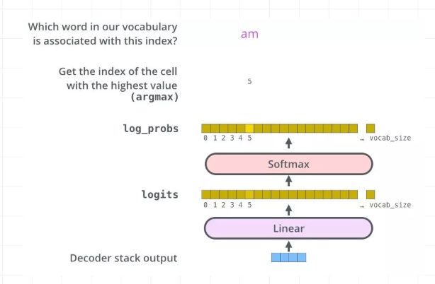
这里,我们直接给出代码:
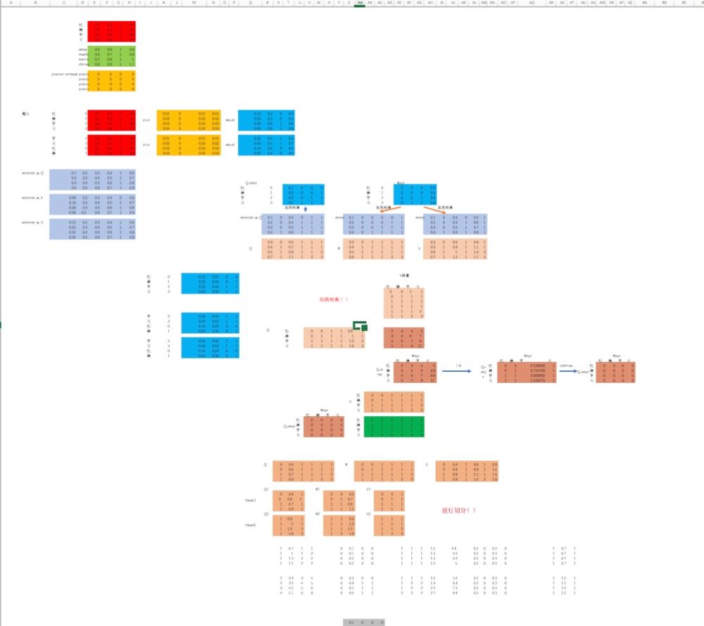
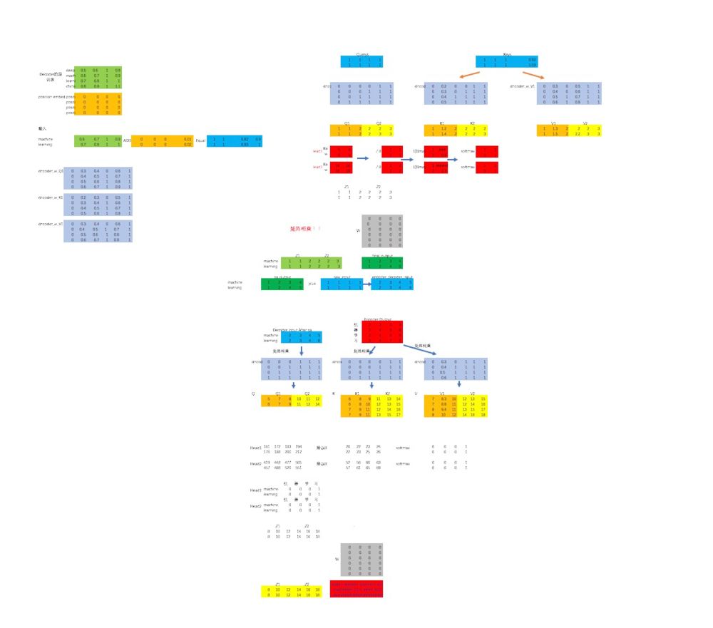
W_final = tf.constant([[0.2,0.3,0.5,0.4], [0.2,0.3,0.5,0.4], [0.2,0.3,0.5,0.4], [0.2,0.3,0.5,0.4]])logits = tf.matmul(tf.reshape(decoder_outputs,(-1,tf.shape(decoder_outputs)[2])),W_final)logits = tf.reshape(logits,(tf.shape(decoder_outputs)[0],tf.shape(decoder_outputs)[1],-1)) logits = tf.nn.softmax(logits)y = tf.one_hot(decoder_input,depth=4)loss = tf.nn.softmax_cross_entropy_with_logits(logits=logits,labels=y)train_op = tf.train.AdamOptimizer(learning_rate=0.0001).minimize(loss)整个文章下来,咱们不仅通过excel实现了一遍transorform的正向传播过程,还通过tf代码实现了一遍。放两张excel的抽象图,就知道是多么浩大的工程了:
好了,文章最后,咱们再来回顾一下整个Transformer的结构:
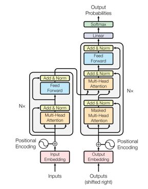
希望通过本文,你能够对Transformer的整体结构有个更清晰的认识!
(*本文为 AI科技大本营转载文章,转载请联系原作者)
◆
精彩推荐
◆
大会开幕倒计时8天!
2019以太坊技术及应用大会特邀以太坊创始人V神与众多海内外知名技术专家齐聚北京,聚焦区块链技术,把握时代机遇,深耕行业应用,共话以太坊2.0新生态。即刻扫码,享优惠票价。


推荐阅读
真正的博士是如何参加AAAI, ICML, ICLR等AI顶会的?
Python最抢手、Java最流行、Go最有前途,7000位程序员揭秘2019软件开发现状
程序员学Python编程或许不知的十大提升工具
不要让 Chrome 成为下一个 IE!
这位博士跑赢“地震波”:提前 10 秒预警宜宾地震!
一张图告诉你到底学Python还是Java!
鸿蒙将至,安卓安否?
25岁创立加密城堡, 曾经独角兽创始人社会名流天才黑客是这里的沙发客, 如今却无人问津……
352万帧标注图片,1400个视频,亮风台推最大单目标跟踪数据集
 你点的每个“在看”,我都认真当成了喜欢
相关文章:

通过注册表修改VC6.0的字体【转】
2019独角兽企业重金招聘Python工程师标准>>> 在VC6.0下更改字体,我们一般通过菜单-Tools-Options-Format来更改 但在我的win7 64位系统下这一选项下的字体和字体颜色是空的,无法选择 所以我想起来通过注册表来更改。 WinR输入“Regedit”&…
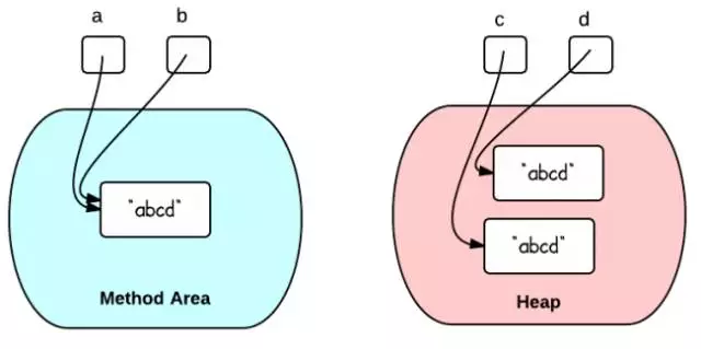
Java中创建String的两种方式差异
我们知道创建一个String类型的变量一般有以下两种方法: String str1 "abcd"; String str2 new String("abcd"); 那么为什么会存在这两种创建方式呢,它们在内存中的表现形式各有什么区别? 方法1: String a …

OpenCV支持的图像格式
OpenCV目前支持的图像格式包括: Windows位图文件 - BMP, DIB; JPEG文件 - JPEG, JPG, JPE; 便携式网络图片 - PNG; 便携式图像格式 - PBM,PGM,PPM; Sun rasters - SR,RASÿ…
Debian Linux下的Python学习——控制流
python中有三种控制流语句:if、for和while。 1. if语句用法( if..elif..else) 代码: 运行: 注意:raw_input函数要求输入一个字符串,int把这个字符串转换为整数 2.for语句用法 (for ... else) 代码: 运行: 注:else部分是可选的。如果包含else,它总是在for循环结束后…
如何运行ImageMagick的命令行工具
在http://www.imagemagick.org/script/index.php网站下载相应的执行文件,这里以下载ImageMagick-6.6.5-10-Q16-windows-static.exe为例说明。 将ImageMagick-6.6.5-10-Q16-windows-static.exe下载后,安装,然后将其中需要的命令行工具考到你需…

华为最强自研NPU问世,麒麟810“抛弃”寒武纪
整理 | 一一出品 | AI科技大本营(ID:rgznai100)“能效高、算子多、精度高”,华为消费者业务手机产品线总裁何刚用一句话总结了自研达芬奇架构给最新麒麟810芯片带来的变化。6 月 21 日,在 HUAWEI Nova 5 系列新品发布会上&#x…
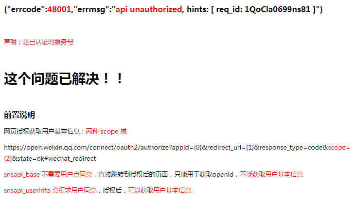
调用 微信接口报错 {errcode:48001,errmsg:api unauthorized, hints: [ req_id: 1QoCla0699ns81 ]}...
如下截图,仅为备份,本文转载地址: http://www.cnblogs.com/liaolongjun/p/6080240.html 以下正文↓↓↓↓↓↓↓↓↓↓↓↓↓↓↓↓↓↓↓↓↓↓↓↓↓↓↓↓↓↓↓↓↓↓↓↓ ↑↑↑↑↑↑↑↑↑↑↑↑↑↑↑↑↑↑↑↑↑↑↑↑↑↑↑↑↑↑…

javascript this用法小结
this是面向对象语言中的一个重要概念,在JAVA,C#等大型语言中,this固定指向运行时的当前对象。但是在javascript中,由于 javascript的动态性(解释执行,当然也有简单的预编译过程),this的指向在运…
在vc6控制台程序中如何调用运行ImageMagick命令行工具
在http://www.imagemagick.org/script/index.php网站下载相应的执行文件,这里以下载ImageMagick-6.6.5-10-Q16-windows-static.exe为例说明。 将ImageMagick-6.6.5-10-Q16-windows-static.exe下载后,安装,然后将其中需要的命令行工具考到你程…
高频数据交换下Flutter与ReactNative的对比
后端使用go写的socketio服务模拟期货行情数据,每10ms推送10条行情数据 ReactNative已经尽力优化了。 Flutter由于没flutter-socketio这个库不支持dart2.0以上的版本,所有用了安卓的socketio,通过事件与Flutter通讯。 1.内存占用 ReactNative …

6月技术福利限时免费领
《程序员大本营》6月刊来啦~更多福利限时免费领取:CSDN重磅技术大会精选视频以及200PPT;机器学习、知识图谱、计算机视觉、区块链等100技术公开课及PPT全奉送...识别海报二维码,邀请3位好友扫码助力,即可免费领取↓↓↓❤提示&…
我对bgwriter.c 与 guc 关系的初步理解
我用例子来说明:只是一个模拟,我自己做的 假的 bgwriter.c [rootlocalhost test]# cat bgwriter.c #include<stdio.h> #include<stdlib.h> #include<signal.h> #include "bgwriter.h" #include "guc.h" //some co…

媲美Pandas?一文入门Python的Datatable操作
作者 | Parul Pandey译者 | linstancy责编 | Jane出品 | Python大本营(id:pythonnews)【导读】工具包 datatable 的功能特征与 Pandas 非常类似,但更侧重于速度以及对大数据的支持。此外,datatable 还致力于实现更好的…
java并发编程——并发容器类介绍
2019独角兽企业重金招聘Python工程师标准>>> 并发容器的简单介绍 JDK5中添加了新的concurrent包,相对同步容器而言,并发容器通过一些机制改进了并发性能。因为同步容器将所有对容器状态的访问都串行化了,这样保证了线程的安全性&a…
CV_IMAGE_ELEM参数赋值时注意的问题
转自:http://hi.baidu.com/wangruiy01/blog/item/041ab03e8abd33c57d1e71a0.html CV_IMAGE_ELEM是一个宏, #define CV_IMAGE_ELEM( image, elemtype, row, col ) /(((elemtype*)((image)->imageData (image)->widthStep*(row)))[(col)])#define …
公司内部exchange2010 下删除误发邮件
1、Add-PSSnapin Microsoft.Exchange.Management.PowerShell.E20102、get-mailbox | search-mailbox -SearchQuery 填写误发邮件标题 -TargetMailbox "administrator" -TargetFolder "SearchAndDeleteLog" -DeleteContent转载于:https://blog.51cto.com/wo…

从代码设计到应用开发,入坑深度学习看这本书就够了
深度学习(Deep Learning)是机器学习中一种基于对数据进行表征学习的方法。近年来,深度学习已经在科技界、工业界日益广泛地应用。随着全球各领域多样化数据的极速积累和计算资源的成熟化商业服务,深度学习已经成为人工智能领域最有…
小波矩特征提取matlab代码
这是我上研究生时写的小波矩特征提取代码: %新归一化方法小波矩特征提取---------------------------------------------------------- Fimread(a1.bmp);Fim2bw(F);Fimresize(F,[128 128]);%求取最上点for i1:128 for j1:128 if (F(i,j)1) yt…
hadoop生态搭建(3节点)-06.hbase配置
# http://archive.apache.org/dist/hbase/1.2.4/ # 安装 hbase tar -zxvf ~/hbase-1.2.4-bin.tar.gz -C /usr/local rm –r ~/hbase-1.2.4-bin.tar.gz # 配置环境变量# node1 node2 node3 vi /etc/profile# 在export PATH USER LOGNAME MAIL HOSTNAME HISTSIZE HISTCONTROL下添…

异类框架BigDL,TensorFlow的潜在杀器!
作者 | Nandita Dwivedi译者 | 风车云马责编 | Jane出品 | AI 科技大本营(id:rgznai100)【导读】你能利用现有的 Spark 集群构建深度学习模型吗?如何分析存储在 HDFS、Hive 和 HBase 中 tb 级的数据吗?企业想用深度学习…
对IsUnderPostmaster变量初步学习
开始 在postmaster.c 中的 BackendStartup 中,有如下的代码: 其中定义了 IsUnderPostmastertrue。 而bgwriter 作为 postmaster 的子进程,它的 IsUnderPostmaster 也是为真。 * BackendStartup -- start backend process** returns: STATUS_…
C++读写ini配置文件GetPrivateProfileString()WritePrivateProfileString()
转自:http://hi.baidu.com/andywangcn/blog/item/10ba730f48160eeb37d122e9.html 配置文件中经常用到ini文件,在VC中其函数分别为: #include <Windows.h> //wince,WMobile.ppc不支持这几个函数 写入.ini文件:bool WritePriv…
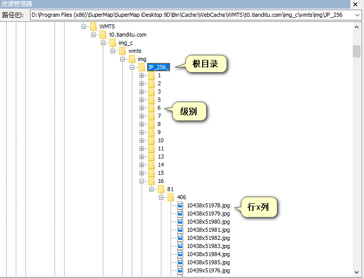
地图下载2之天超图瓦片格式
接上一篇《地图下载1之天地图瓦片解析》,我们已经知道了天地图的瓦片格式,现在来分析一下超图中瓦片的存储结构。 其实,在GIS领域,只有像ESRI这样强大公司的SHP文件等能通用外,很多数据、格式等都不通用,都…
server 2003登录界面黑屏的解决办法
1、备份注册表(为了安全起见)具体办法:开始-> 运行窗口输入“regedit.exe”->回车->找到注册表->文件->导出->完成; 2、复制下面的文件内容到记事本然后另存为格式为.reg注册表扩展名导入注册表; Wi…

“学了半年后,我要揭开Python 3宗罪!”
有人曾说,未来只有2种人,会Python的人和....不懂Python的小学生,虽有夸张,这也意味着Python越来越重要了,究竟这门语言厉害在哪里?以下为你总结了Python3宗“罪”!Python凭啥这么优秀࿱…
连表/子查询/计算的sql
看不懂的sql语句 1.select om.*,money,cus.c_type,cus.c_weixin_name,isnull(cus.c_discount,0) c_discount,isnull(om.o_money-om.o_money*cus.c_discount,0) money1,isnull(money*(i_year_pointi_month_potinti_piece_point),0) money2,isnull((om.o_money-om.o_money*cus.c_…
vc6静态库的生成和调用
1、静态库的生成: 在vc6.0中CtrlN选择Projects下的Win32 Static Library,Project name:SumLib,点击OK,下一页中的两项可选可不选,点击Finish完成。 在此工程中新建lib.h和lib.cpp两个文件,源码如下: //lib.…

实例变量的访问及数据封装
你已经看到处理分数的方法如何通过名称直接访问两个实例变量numerator和denominator。事实上,实例方法总是可以直接访问它的实例变量的。然而,类方法则不能,因为它只处理本身,并不处理任何类实例(仔细想想)…

清华成立视觉智能研究中心,邓志东任中心主任
整理 | 阿司匹林出品 | AI科技大本营(ID: rgznai100)6月21日,清华大学人工智能研究院视觉智能研究中心正式成立,清华大学副校长、清华大学人工智能研究院管委会主任尤政院士,清华大学人工智能研究院院长张钹院士出席成…

Java并发编程(一)Thread详解
一、概述 在开始学习Thread之前,我们先来了解一下 线程和进程之间的关系: 线程(Thread)是进程的一个实体,是CPU调度和分派的基本单位。 线程不能够独立执行,必须依存在应用程序中,由应用程序提供多个线程执行控制。 线…