作者 | Matthew Stewart

译者 | Monanfei

责编 | Jane

出品 | AI科技大本营（ID: rgznai100）

【导读】在本文中，我们将为大家介绍如何对神经网络的超参数进行优化调整，以便在 Beale 函数上获得更高性能，Beale 函数是评价优化有效性的众多测试函数之一。

Beale 函数

当应用数学家开发一种新的优化算法时，常用的做法是在测试函数上测试该算法，主要的评价指标如下：

• 收敛速度（求得解的速度有多快）

• 精度（接近真值的距离有多远）

• 稳健性（在整体上表现良好，还是仅在一部分上表现较好）

• 一般性能（例如计算复杂性等）

Beale 函数的可视化如下：

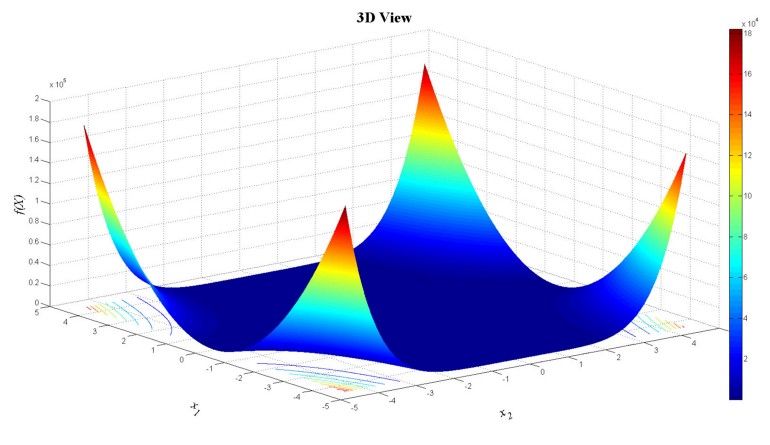
Beale 函数评估了在非常浅梯度的平坦区域中优化算法的表现。在这种情况下，基于梯度的优化程序很难达到最小值，因为它们无法有效地进行学习。

Beale 函数的曲面类似于神经网络的损失表面，在训练神经网络时，希望通过执行某种形式的优化来找到损失表面上的全局最小值 ，而最常采用的方法就是随机梯度下降。

首先定义 Beale 函数：

# define Beale's function which we want to minimize	
def objective(X):	x = X[0]; y = X[1]	return (1.5 - x + x*y)**2 + (2.25 - x + x*y**2)**2 + (2.625 - x + x*y**3)**2

接下来设置 Beale 函数的边界，以及格网的步长：

# function boundaries	
xmin, xmax, xstep = -4.5, 4.5, .9	
ymin, ymax, ystep = -4.5, 4.5, .9

然后，根据上述设置来制作格网，并准备寻找函数最小值

# Let's create some points	
x1, y1 = np.meshgrid(np.arange(xmin, xmax + xstep, xstep), np.arange(ymin, ymax + ystep, ystep))

我们先做一个初步猜测（通常很糟糕）

# initial guess	
x0 = [4., 4.]	
f0 = objective(x0)	
print (f0)

然后使用 scipy.optimize.minimize 函数并查看优化结果

bnds = ((xmin, xmax), (ymin, ymax))	
minimum = minimize(objective, x0, bounds=bnds)	
print(minimum)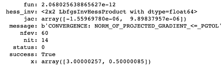

神经网络中的优化

神经网络的优化可以定义为如下的过程：网络预测——计算误差——再次预测测——试图最小化这个误差——再次预测...——直到误差不再降低。

在神经网络中，最常用的优化算法是梯度下降，梯度下降中使用的目标函数就是想要最小化的损失函数。

由于本教程的神经网络构建和优化过程是基于 Keras 搭建，所以在介绍优化过程之前，我们先回顾一下 Keras 的基本内容, 这将有助于理解后续的优化操作。

Keras 简介

Keras 是一个深度学习的 Python 库，它旨在快速简便地开发深度学习模型。Keras 建立在模型的基础上。Keras 有两种构建模型的方式，一种是 Sequential 模型，它是神经网络层的线性堆栈。另一种是 基于函数 API 构建模型，这是一种定义复杂模型的方法。

以 Sequential 方式为例，构建 Keras 深度学习模型的流程如下：

1. 定义模型：创建 Sequential 模型并添加网络层。

2. 编译模型：指定损失函数和优化器，并调用 .compile() 函数对模型进行编译。

3. 模型训练：通过调用 .fit() 函数在数据上训练模型。

4. 进行预测：调用 .evaluate() 或 .predict() 函数来对新数据进行预测。

   
   

为了在模型运行时检查模型的性能，需要用到回调函数（callbacks）

回调函数：在训练时记录模型性能

回调是在训练过程的给定阶段执行的一组函数，可以使用回调来获取训练期间模型内部状态和模型统计信息的视图。常用的回调函数如下：

1. keras.callbacks.History() 记录模型训练的历史信息，该函数默认包含在 .fit() 中

2. keras.callbacks.ModelCheckpoint()将模型的权重保存在训练中的某个节点。如果模型运行了很长时间并且中途可能发生系统故障，该函数将非常有用。

3. keras.callbacks.EarlyStopping()当监控值停止改善时停止训练

4. keras.callbacks.LearningRateScheduler() 在训练过程中改变学习率

接下来导入 keras 中一些必要的库和函数：

import tensorflow as tf	
import keras	
from keras import layers	
from keras import models	
from keras import utils	
from keras.layers import Dense	
from keras.models import Sequential	
from keras.layers import Flatten	
from keras.layers import Dropout	
from keras.layers import Activation	
from keras.regularizers import l2	
from keras.optimizers import SGD	
from keras.optimizers import RMSprop	
from keras import datasets	from keras.callbacks import LearningRateScheduler	
from keras.callbacks import History	from keras import losses	
from sklearn.utils import shuffle	print(tf.VERSION)	
print(tf.keras.__version_

如果希望网络使用随机数工作，而且期望结果可以复现，可以使用随机种子，相同的随机种子每次都会产生相同的数字序列。

# fix random seed for reproducibility	
np.random.seed(5)

第一步：确定网络的拓扑结构

使用 MNIST 数据集进行实验，该数据集由 28x28 手写数字（0-9）的灰度图像组成。每个像素为 8 位，取值范围为 0 到 255。获取数据的代码如下：

mnist = keras.datasets.mnist	
（x_train，y_train），（x_test，y_test）= mnist.load_data（）	
x_train.shape，y_train.shape

X 和 Y 的尺寸分别为（60000,28,28）和（60000,1），我们可以使用如下代码来可视化数据集：

plt.figure(figsize=(10,10))	
for i in range(10):	plt.subplot(5,5,i+1)	plt.xticks([])	plt.yticks([])	plt.grid(False)	plt.imshow(x_train[i], cmap=plt.cm.binary)	plt.xlabel(y_train[i])

最后，我查一下训练集和测试集的维度：

print(f'We have {x_train.shape[0]} train samples')	
print(f'We have {x_test.shape[0]} test samples')

我们一共有60,000张训练图像和10,000张测试图像，接下来要对数据进行预处理。

数据预处理

• 首先，需要将 2D 图像转为 1D序列（展平），numpy.reshape()和 keras.layers.Flatten都可以实现展平操作。

• 然后，使用如下公式来对数据进行标准化（0~1 标准化）

在本例中，最小值为 0，最大值为255，因此公式简化为 ?：=? / 255，代码如下：

# normalize the data	
x_train, x_test = x_train / 255.0, x_test / 255.0	# reshape the data into 1D vectors	
x_train = x_train.reshape(60000, 784)	
x_test = x_test.reshape(10000, 784)	num_classes = 10	# Check the column length	
x_train.shape[1]

接下来对数据进行 one-hot 编码

# Convert class vectors to binary class matrices	
y_train = keras.utils.to_categorical(y_train, num_classes)	
y_test = keras.utils.to_categorical(y_test, num_classes)est，num_classes）

最后，就可以构建自己的模型了。

第二步：调整学习率

最常见的优化算法之一是随机梯度下降（SGD），SGD中可以进行优化的超参数有 learning rate，momentum，decay 和 nesterov。

Learning rate 控制每个 batch 结束时的模型权重，momentum控制先前权重更新对当前权重更新的影响程度，decay表示每次更新时的学习率衰减，nesterov 用于选择是否要使用 Nesterov动量，其取值为 “True” 或 “False” 。

这些超参数的典型值是 lr = 0.01，decay = 1e-6，momentum = 0.9，nesterov = True。

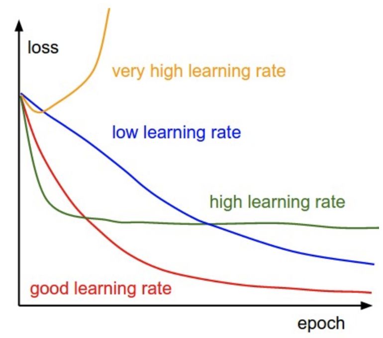
在训练过程中，不同学习率对 loss 的影响如下图所示：

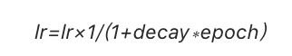
Keras 在 SGD 优化器中具有默认的学习率调整器，该调整器根据随机梯度下降优化算法，在训练期间降低学习速率，学习率的调整公式如下：

接下来，我们将在 Keras 中实现学习率调整。将学习率的初始值设置为 0.1，然后将学习率衰减设为 0.0016，并将模型训练 60 个 epochs。此外，将动量值设为 0.8 。

epochs=60	
learning_rate = 0.1	
decay_rate = learning_rate / epochs	
momentum = 0.8	sgd = SGD(lr=learning_rate, momentum=momentum, decay=decay_rate, nesterov=False)

构建神经网络模型：

# build the model	
input_dim = x_train.shape[1]	lr_model = Sequential()	
lr_model.add(Dense(64, activation=tf.nn.relu, kernel_initializer='uniform',	input_dim = input_dim))	
lr_model.add(Dropout(0.1))	
lr_model.add(Dense(64, kernel_initializer='uniform', activation=tf.nn.relu))	
lr_model.add(Dense(num_classes, kernel_initializer='uniform', activation=tf.nn.softmax))	# compile the model	
lr_model.compile(loss='categorical_crossentropy',	optimizer=sgd,	metrics=['acc']

下面进行模型训练：

%%time	
# Fit the model	
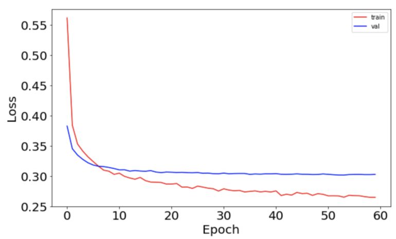
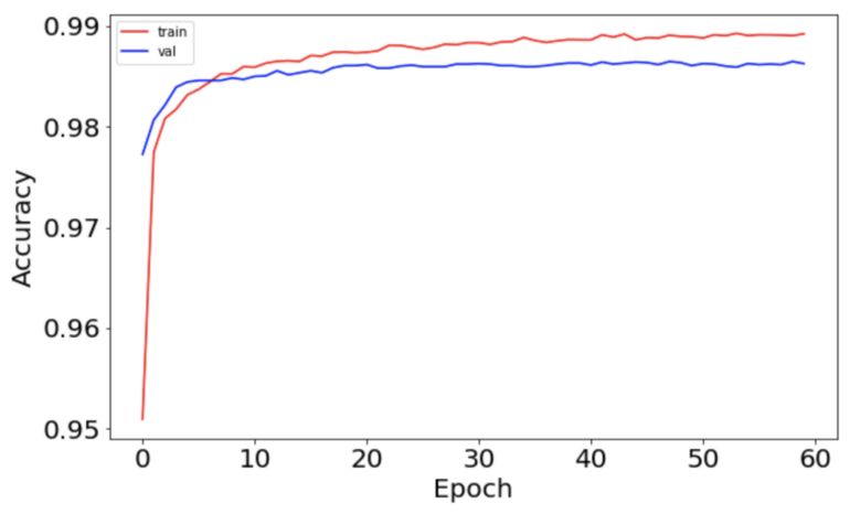
batch_size = int(input_dim/100)	lr_model_history = lr_model.fit(x_train, y_train,	batch_size=batch_size,	epochs=epochs,	verbose=1,	validation_data=(x_test, y_test))

模型训练完成后，画出精度和误差随 epoch 变化的曲线：

# Plot the loss function	
fig, ax = plt.subplots(1, 1, figsize=(10,6))	
ax.plot(np.sqrt(lr_model_history.history['loss']), 'r', label='train')	
ax.plot(np.sqrt(lr_model_history.history['val_loss']), 'b' ,label='val')	
ax.set_xlabel(r'Epoch', fontsize=20)	
ax.set_ylabel(r'Loss', fontsize=20)	
ax.legend()	
ax.tick_params(labelsize=20)	# Plot the accuracy	
fig, ax = plt.subplots(1, 1, figsize=(10,6))	
ax.plot(np.sqrt(lr_model_history.history['acc']), 'r', label='train')	
ax.plot(np.sqrt(lr_model_history.history['val_acc']), 'b' ,label='val')	
ax.set_xlabel(r'Epoch', fontsize=20)	
ax.set_ylabel(r'Accuracy', fontsize=20)	
ax.legend()	
ax.tick_params(labelsize=20)

误差曲线如下图所示：

精度曲线如下：

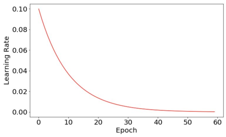
使用 LearningRateScheduler 对学习率进行调节

我们可以定制一个指数衰减的学习率调整器：

??=??₀ × ?^(−??)

该过程和上节中的过程非常相似，为了比较两者的差异，将两者的代码写在一起，如下所示：

# solution	
epochs = 60	
learning_rate = 0.1 # initial learning rate	
decay_rate = 0.1	
momentum = 0.8	# define the optimizer function	
sgd = SGD(lr=learning_rate, momentum=momentum, decay=decay_rate, nesterov=False)	input_dim = x_train.shape[1]	
num_classes = 10	
batch_size = 196

# build the model	
exponential_decay_model = Sequential()	
exponential_decay_model.add(Dense(64, activation=tf.nn.relu, kernel_initializer='uniform', input_dim = input_dim))	
exponential_decay_model.add(Dropout(0.1))	
exponential_decay_model.add(Dense(64, kernel_initializer='uniform', activation=tf.nn.relu))	
exponential_decay_model.add(Dense(num_classes, kernel_initializer='uniform', activation=tf.nn.softmax)

# compile the model	
exponential_decay_model.compile(loss='categorical_crossentropy',	optimizer=sgd,	metrics=['acc'])	
# define the learning rate change	
def exp_decay(epoch):	lrate = learning_rate * np.exp(-decay_rate*epoch)	return lrate

# learning schedule callback	
loss_history = History()	
lr_rate = LearningRateScheduler(exp_decay)	
callbacks_list = [loss_history, lr_rate]	# you invoke the LearningRateScheduler during the .fit() phase	
exponential_decay_model_history = exponential_decay_model.fit(x_train, y_train,	batch_size=batch_size,	epochs=epochs,	callbacks=callbacks_list,	verbose=1,	validation_data=(x_test, y_test))	

可以发现，两者唯一的区别就是 exp_decay的有无，以及是否在 LearningRateScheduler 中调用。我们可以画出使用 exp_decay的模型的学习率曲线，学习率的衰减过程显得很平滑，如下图所示：

误差的变化曲线也变得更加平滑：

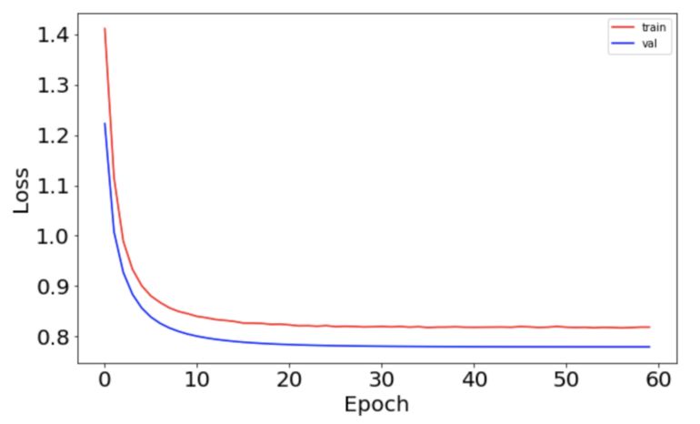
从上述曲线中我们看出，使用合适的学习率衰减策略，有利于提高神经网络的性能。

第三步：选择优化器（optimizer）和误差函数（loss function）

在构建模型并使用它来进行预测时，通过定义损失函数（或 目标函数）来衡量预测结果的好坏。 

在某些情况下，损失函数和距离测量有关。 距离测量方式取决于数据类型和正在处理的问题。例如，在自然语言处理（分析文本数据）中，汉明距离的使用最为常见。

距离度量

• 欧式距离

• 曼哈顿距离

• 其他距离，如汉明距离等

损失函数

• MSE（回归问题）

• 分类交叉熵（分类问题）

• 二元交叉熵（分类问题）

# build the model	
input_dim = x_train.shape[1]	model = Sequential()	
model.add(Dense(64, activation=tf.nn.relu, kernel_initializer='uniform',	input_dim = input_dim)) # fully-connected layer with 64 hidden units	
model.add(Dropout(0.1))	
model.add(Dense(64, kernel_initializer='uniform', activation=tf.nn.relu))	
model.add(Dense(num_classes, kernel_initializer='uniform', activation=tf.nn.softmax))	# defining the parameters for RMSprop (I used the keras defaults here)	
rms = RMSprop(lr=0.001, rho=0.9, epsilon=None, decay=0.0)	model.compile(loss='categorical_crossentropy',	optimizer=rms,	metrics=['acc'])

第四步：决定 batch 大小和 epoch 的次数

batch 大小决定了每次前向传播中的样本数目。使用 batch 的好处如下（前提是 batch size 小于样本总数）：

• 需要的内存更少。 由于使用较少的样本训练网络，因此整体训练过程需要较少的内存。 如果数据集太大，无法全部放入机器的内存中，那么使用 batch 显得尤为重要。

• 一般来讲，网络使用较小的 batch 来训练更快。这是因为在每次前向传播后，网络都会更新一次权重。

epoch 的次数决定了学习算法对整个训练数据集的迭代次数。

一个 epoch 将训练数据集中的每个样本，一个 epoch 由一个或多个 batch 组成。选择 batch 大小或 epoch 的次数没有硬性的限制，而且增加 epoch 次数并不能保证取得更好的结果。

%%time	
batch_size = input_dim	
epochs = 60	model_history = model.fit(x_train, y_train,	batch_size=batch_size,	epochs=epochs,	verbose=1,	validation_data=(x_test, y_test))

score = model.evaluate(x_test, y_test, verbose=0)	
print('Test loss:', score[0])	
print('Test accuracy:', score[1])	fig, ax = plt.subplots(1, 1, figsize=(10,6))	
ax.plot(np.sqrt(model_history.history['acc']), 'r', label='train_acc')	
ax.plot(np.sqrt(model_history.history['val_acc']), 'b' ,label='val_acc')	
ax.set_xlabel(r'Epoch', fontsize=20)	
ax.set_ylabel(r'Accuracy', fontsize=20)	
ax.legend()	
ax.tick_params(labelsize=20)	fig, ax = plt.subplots(1, 1, figsize=(10,6))	
ax.plot(np.sqrt(model_history.history['loss']), 'r', label='train')	
ax.plot(np.sqrt(model_history.history['val_loss']), 'b' ,label='val')	
ax.set_xlabel(r'Epoch', fontsize=20)	
ax.set_ylabel(r'Loss', fontsize=20)	
ax.legend()	
ax.tick_params(labelsize=20)

第五步：随机重启

该方法在keras中没有直接的实现，我们可以通过更改 keras.callbacks.LearningRateScheduler 来实现，它主要用于在一定 epoch 之后重置有限次 epoch 的学习率。

使用交叉验证来调节超参数

使用 Scikit-Learn 的 GridSearchCV ，可以自动计算超参数的几个可能值，并比较它们的结果。

为了使用 keras 进行交叉验证，可以使用 Scikit-Learn API 的包装器，该包装器使得 Sequential 模型（仅支持单输入）成为 Scikit-Learn 工作流的一部分。

有两个包装器可供使用：

• keras.wrappers.scikit_learn.KerasClassifier(build_fn=None, **sk_params)，它实现了Scikit-Learn 分类器接口。

• keras.wrappers.scikit_learn.KerasRegressor(build_fn=None, **sk_params)，它实现了Scikit-Learn 回归器接口。

import numpy	
from sklearn.model_selection import GridSearchCV	
from keras.wrappers.scikit_learn import KerasClassifier

尝试不同的权重初始值

# let's create a function that creates the model (required for KerasClassifier)	
# while accepting the hyperparameters we want to tune	
# we also pass some default values such as optimizer='rmsprop'	
def create_model(init_mode='uniform'):	# define model	model = Sequential()	model.add(Dense(64, kernel_initializer=init_mode, activation=tf.nn.relu, input_dim=784))	model.add(Dropout(0.1))	model.add(Dense(64, kernel_initializer=init_mode, activation=tf.nn.relu))	model.add(Dense(10, kernel_initializer=init_mode, activation=tf.nn.softmax))	# compile model	model.compile(loss='categorical_crossentropy',	optimizer=RMSprop(),	metrics=['accuracy'])	return model

%%time	
seed = 7	
numpy.random.seed(seed)	
batch_size = 128	
epochs = 10	model_CV = KerasClassifier(build_fn=create_model, epochs=epochs,	batch_size=batch_size, verbose=1)

# define the grid search parameters	
init_mode = ['uniform', 'lecun_uniform', 'normal', 'zero',	'glorot_normal', 'glorot_uniform', 'he_normal', 'he_uniform']	
param_grid = dict(init_mode=init_mode)	
grid = GridSearchCV(estimator=model_CV, param_grid=param_grid, n_jobs=-1, cv=3)	
grid_result = grid.fit(x_train, y_train)

# print results	
print(f'Best Accuracy for {grid_result.best_score_} using {grid_result.best_params_}')	
means = grid_result.cv_results_['mean_test_score']	
stds = grid_result.cv_results_['std_test_score']	
params = grid_result.cv_results_['params']	
for mean, stdev, param in zip(means, stds, params):	print(f' mean={mean:.4}, std={stdev:.4} using {param}')

GridSearch 的结果如下：

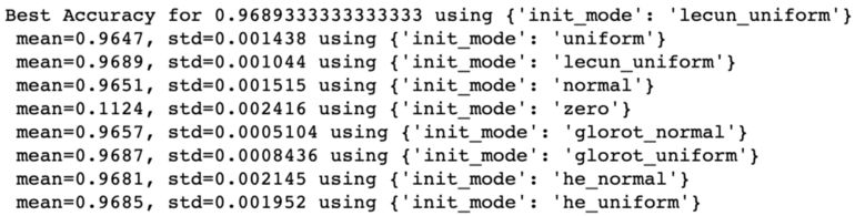
可以看到最好的结果是使用 lecun_uniform 初始化或 glorot_uniform 初始化，在这两种初始化的基础上，我们的网络取得了接近 97％ 的准确度。

将模型保存到 JSON 文件中

分层数据格式（HDF5）是用于存储大数组的数据存储格式，这包括神经网络中权重的值。HDF5 的安装可以使用如下命令 ：pip install h5py

Keras 使用JSON格式保存模型的代码如下：

from keras.models import model_from_json	# serialize model to JSON	
model_json = model.to_json()	with open("model.json", "w") as json_file:	json_file.write(model_json)	# save weights to HDF5	
model.save_weights("model.h5")	
print("Model saved")	# when you want to retrieve the model: load json and create model	
json_file = open('model.json', 'r')	
saved_model = json_file.read()	
# close the file as good practice	
json_file.close()	
model_from_json = model_from_json(saved_model)	
# load weights into new model	
model_from_json.load_weights("model.h5")	
print("Model loade")

对多个超参数同时进行交叉验证

使用 GridSearch，可以同时对多个参数进行交叉验证，并有效地尝试它们的组合。

例如，可以搜索以下参数的不同的取值：

• batch 大小

• epoch 次数

• 初始模式

这些选项将被指定到字典中，该字典将传递给 GridSearchCV。

注意：神经网络中的交叉验证在计算上是很昂贵的，每个组合都将使用 k 折交叉验证评估。

# repeat some of the initial values here so we make sure they were not changed	
input_dim = x_train.shape[1]	
num_classes = 10	# let's create a function that creates the model (required for KerasClassifier)	
# while accepting the hyperparameters we want to tune	
# we also pass some default values such as optimizer='rmsprop'	
def create_model_2(optimizer='rmsprop', init='glorot_uniform'):	model = Sequential()	model.add(Dense(64, input_dim=input_dim, kernel_initializer=init, activation='relu'))	model.add(Dropout(0.1))	model.add(Dense(64, kernel_initializer=init, activation=tf.nn.relu))	model.add(Dense(num_classes, kernel_initializer=init, activation=tf.nn.softmax))	# compile model	model.compile(loss='categorical_crossentropy',	optimizer=optimizer,	metrics=['accuracy'])	return mode

%%time	
# fix random seed for reproducibility (this might work or might not work	
# depending on each library's implenentation)	
seed = 7	
numpy.random.seed(seed)

# create the sklearn model for the network	
model_init_batch_epoch_CV = KerasClassifier(build_fn=create_model_2, verbose=1)	# we choose the initializers that came at the top in our previous cross-validation!!	
init_mode = ['glorot_uniform', 'uniform']	
batches = [128, 512]	
epochs = [10, 20]

‍

# grid search for initializer, batch size and number of epochs	
param_grid = dict(epochs=epochs, batch_size=batches, init=init_mode)	
grid = GridSearchCV(estimator=model_init_batch_epoch_CV, 	param_grid=param_grid,	cv=3)	
grid_result = grid.fit(x_train, y_train)

# print results	
print(f'Best Accuracy for {grid_result.best_score_:.4} using {grid_result.best_params_}')	
means = grid_result.cv_results_['mean_test_score']	
stds = grid_result.cv_results_['std_test_score']	
params = grid_result.cv_results_['params']	
for mean, stdev, param in zip(means, stds, params):	print(f'mean={mean:.4}, std={stdev:.4} using {param}')

在结束之前，还有留有最后一个问题：如果在 GridSearchCV 中，需要搜索的参数量和取值空间都特别大，我们该怎么办？

这是一个特别麻烦的问题，想象一下，假设要优化 5 个参数，每个参数有 10 个潜在值，那么组合数将是 10⁵，这意味着我们必须训练一个非常大的网络。 显然，这种方式不切实际，所以通常使用 RandomizedCV 作为替代方案。

RandomizedCV 允许指定所有的潜在参数，然后在交叉验证中的每折中，它将选择参数的一个随机子集，对该子集进行验证。 最后，可以选择最佳的参数集并将其作为近似解。

原文链接： 

https://towardsdatascience.com/simple-guide-to-hyperparameter-tuning-in-neural-networks-3fe03dad8594

（*本文为 AI科技大本营编译文章，转载请联系1092722531）

◆

精彩推荐

◆

“只讲技术，拒绝空谈！”2019 AI开发者大会将于9月6日-7日在北京举行，这一届AI开发者大会有哪些亮点？一线公司的大牛们都在关注什么？AI行业的风向是什么？2019 AI开发者大会，倾听大牛分享，聚焦技术实践，和万千开发者共成长。

目前，大会盲订票限量发售中~扫码购票，领先一步！

推荐阅读

• 码农们的「血与泪」：新零售「全渠道中台」的前世今身

• 腾讯拥抱开源：首次公布开源路线图，技术研发向共享、复用和开源迈进

• 混合云发展之路：前景广阔，巨头混战

• 干货 | Python后台开发的高并发场景优化解决方案

• 5G 浪潮来袭！程序员在风口中有何机遇？

• 这次又坑多少人? 深度解析 Dash 钱包"关键"漏洞!

• 壕！两万多名腾讯员工获 51 万港元股票奖励