一、前向计算和反向传播数学过程讲解
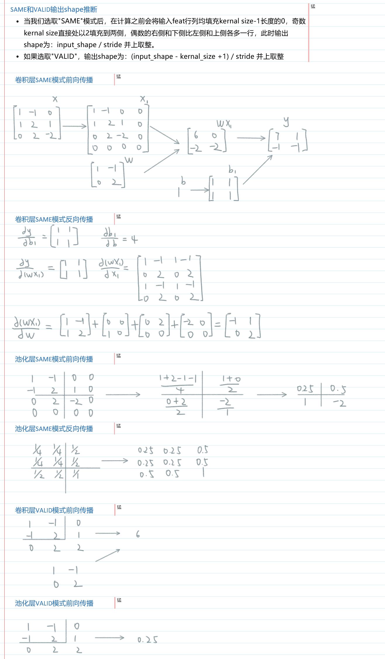
这里讲解的是平均池化层,最大池化层见本文第三小节
二、测试代码
数据和上面完全一致,自行打印验证即可。
1、前向传播
import tensorflow as tf
import numpy as np# 输入张量为3×3的二维矩阵
M = np.array([[[1], [-1], [0]],[[-1], [2], [1]],[[0], [2], [-2]]
])
# 定义卷积核权重和偏置项。由权重可知我们只定义了一个2×2×1的卷积核
filter_weight = tf.get_variable('weights', [2, 2, 1, 1], initializer=tf.constant_initializer([[1, -1],[0, 2]]))
biases = tf.get_variable('biases', [1], initializer=tf.constant_initializer(1))# 调整输入格式符合TensorFlow要求
M = np.asarray(M, dtype='float32')
M = M.reshape(1, 3, 3, 1)# 计算输入张量通过卷积核和池化滤波器计算后的结果
x = tf.placeholder('float32', [1, None, None, 1])# 我们使用了带Padding,步幅为2的卷积操作,因为filter_weight的深度确定了卷积核的数量
conv = tf.nn.conv2d(x, filter_weight, strides=[1, 2, 2, 1], padding='SAME')
bias = tf.nn.bias_add(conv, biases)# 使用带Padding,步幅为2的平均池化操作
pool = tf.nn.avg_pool(x, ksize=[1, 2, 2, 1], strides=[1, 2, 2, 1], padding='VALID')# 执行计算图
with tf.Session() as sess:tf.global_variables_initializer().run()convoluted_M = sess.run(bias, feed_dict={x: M})pooled_M = sess.run(pool, feed_dict={x: M})print("convoluted_M: \n", convoluted_M)print("pooled_M: \n", pooled_M)
2、反向传播
import tensorflow as tf
import numpy as np# 输入张量为3×3的二维矩阵
M = np.array([[[1], [-1], [0]],[[-1], [2], [1]],[[0], [2], [-2]]
])
# 定义卷积核权重和偏置项。由权重可知我们只定义了一个2×2×1的卷积核
filter_weight = tf.get_variable('weights', [2, 2, 1, 1], initializer=tf.constant_initializer([[1, -1],[0, 2]]))
biases = tf.get_variable('biases', [1], initializer=tf.constant_initializer(1))# 调整输入格式符合TensorFlow要求
M = np.asarray(M, dtype='float32')
M = M.reshape(1, 3, 3, 1)# 计算输入张量通过卷积核和池化滤波器计算后的结果
x = tf.placeholder('float32', [1, None, None, 1])# 我们使用了带Padding,步幅为2的卷积操作,因为filter_weight的深度确定了卷积核的数量
conv = tf.nn.conv2d(x, filter_weight, strides=[1, 2, 2, 1], padding='SAME')
bias = tf.nn.bias_add(conv, biases)d_filter = tf.gradients(bias,filter_weight)
d_biases = tf.gradients(bias,biases)
d_conv = tf.gradients(bias,conv)
d_conv_x = tf.gradients(conv,x)
d_conv_w = tf.gradients(conv,filter_weight)
# d_bias_x = tf.gradients(bias,x)# 使用带Padding,步幅为2的平均池化操作
pool = tf.nn.avg_pool(x, ksize=[1, 2, 2, 1], strides=[1, 2, 2, 1], padding='SAME')d_pool = tf.gradients(pool,x)# 执行计算图
with tf.Session() as sess:tf.global_variables_initializer().run()# convoluted_M = sess.run(bias, feed_dict={x: M})# pooled_M = sess.run(pool, feed_dict={x: M})## print("convoluted_M: \n", convoluted_M)# print("pooled_M: \n", pooled_M)print("d_filter:\n", sess.run(d_filter, feed_dict={x: M}))print("d_biases:\n", sess.run(d_biases, feed_dict={x: M}))print("d_conv:\n", sess.run(d_conv, feed_dict={x: M}))print("d_conv_x:\n", sess.run(d_conv_x, feed_dict={x: M}))print("d_conv_w:\n", sess.run(d_conv_w, feed_dict={x: M}))
四、CS31n上实现的卷积层池化层API
1、卷积层
卷积层向前传播示意图:

def conv_forward_naive(x, w, b, conv_param):"""A naive implementation of the forward pass for a convolutional layer.The input consists of N data points, each with C channels, height H and widthW. We convolve each input with F different filters, where each filter spansall C channels and has height HH and width HH.Input:- x: Input data of shape (N, C, H, W)- w: Filter weights of shape (F, C, HH, WW)- b: Biases, of shape (F,)- conv_param: A dictionary with the following keys:- 'stride': The number of pixels between adjacent receptive fields in thehorizontal and vertical directions.- 'pad': The number of pixels that will be used to zero-pad the input.Returns a tuple of:- out: Output data, of shape (N, F, H', W') where H' and W' are given byH' = 1 + (H + 2 * pad - HH) / strideW' = 1 + (W + 2 * pad - WW) / stride- cache: (x, w, b, conv_param)"""out = None############################################################################## TODO: Implement the convolutional forward pass. ## Hint: you can use the function np.pad for padding. #############################################################################pad = conv_param['pad'] stride = conv_param['stride']N, C, H, W = x.shapeF, _, HH, WW = w.shapeH0 = 1 + (H + 2 * pad - HH) / strideW0 = 1 + (W + 2 * pad - WW) / stridex_pad = np.pad(x, ((0,0),(0,0),(pad,pad),(pad,pad)),'constant') # 填充后的输入out = np.zeros((N,F,H0,W0)) # 初始化的输出# 以输出的每一个像素点为单位写出其前传表达式for n in range(N):for f in range(F):for h0 in range(H0):for w0 in range(W0):out[n,f,h0,w0] = np.sum(x_pad[n,:,h0*stride:HH+h0*stride,w0*stride:WW+w0*stride] * w[f]) + b[f]############################################################################## END OF YOUR CODE ##############################################################################cache = (x, w, b, conv_param)return out, cache
卷积层反向传播示意图:

def conv_backward_naive(dout, cache):"""A naive implementation of the backward pass for a convolutional layer.Inputs:- dout: Upstream derivatives.- cache: A tuple of (x, w, b, conv_param) as in conv_forward_naiveReturns a tuple of:- dx: Gradient with respect to x- dw: Gradient with respect to w- db: Gradient with respect to b"""dx, dw, db = None, None, None############################################################################## TODO: Implement the convolutional backward pass. ##############################################################################x, w, b, conv_param = cachepad = conv_param['pad'] stride = conv_param['stride']N, C, H, W = x.shapeF, _, HH, WW = w.shape_, _, H0, W0 = out.shapex_pad = np.pad(x, [(0,0), (0,0), (pad,pad), (pad,pad)], 'constant')dx, dw = np.zeros_like(x), np.zeros_like(w)dx_pad = np.pad(dx, [(0,0), (0,0), (pad,pad), (pad,pad)], 'constant') # 计算b的梯度(F,)db = np.sum(dout, axis=(0,2,3)) # dout:(N,F,H0,W0)# 以每一个dout点为基准计算其两个输入矩阵x(:,:,窗,窗)和w(f)的梯度,注意由于这两个矩阵都是多次参与运算,所以都是累加的关系for n in range(N):for f in range(F):for h0 in range(H0):for w0 in range(W0):x_win = x_pad[n,:,h0*stride:h0*stride+HH,w0*stride:w0*stride+WW]dw[f] += x_win * dout[n,f,h0,w0]dx_pad[n,:,h0*stride:h0*stride+HH,w0*stride:w0*stride+WW] += w[f] * dout[n,f,h0,w0]dx = dx_pad[:,:,pad:pad+H,pad:pad+W]############################################################################## END OF YOUR CODE ##############################################################################return dx, dw, db
2、最大池化层
池化层向前传播:
和卷积层类似,但是更简单一点,只要在对应feature map的原输入上取个窗口然后池化之即可,
def max_pool_forward_naive(x, pool_param):HH, WW = pool_param['pool_height'], pool_param['pool_width']s = pool_param['stride']N, C, H, W = x.shapeH_new = 1 + (H - HH) / sW_new = 1 + (W - WW) / sout = np.zeros((N, C, H_new, W_new))for i in xrange(N): for j in xrange(C): for k in xrange(H_new): for l in xrange(W_new): window = x[i, j, k*s:HH+k*s, l*s:WW+l*s] out[i, j, k, l] = np.max(window)cache = (x, pool_param)return out, cache
池化层反向传播:
反向传播的时候也是还原窗口,除最大值处继承上层梯度外(也就是说本层梯度为零),其他位置置零。
池化层没有过滤器,只有dx梯度,且x的窗口不像卷积层会重叠,所以不用累加,
def max_pool_backward_naive(dout, cache):x, pool_param = cacheHH, WW = pool_param['pool_height'], pool_param['pool_width']s = pool_param['stride']N, C, H, W = x.shapeH_new = 1 + (H - HH) / sW_new = 1 + (W - WW) / sdx = np.zeros_like(x)for i in xrange(N): for j in xrange(C): for k in xrange(H_new): for l in xrange(W_new): window = x[i, j, k*s:HH+k*s, l*s:WW+l*s] m = np.max(window) dx[i, j, k*s:HH+k*s, l*s:WW+l*s] = (window == m) * dout[i, j, k, l]return dx
五、实际框架实现方法
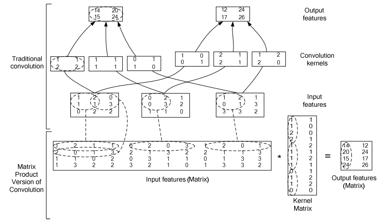
实际框架当然不会才用这种大循环的手段实现卷积操作,矩阵化运算才是正路。
1、Theano
常见的一种拆法是将二维 input 展开成一维向量([in_h * in_w] -> [out_h * out_w]),将卷积核展开为([in_h * in_w, out_h * out_w]),
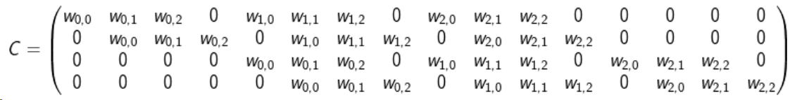
上面仅讨论了2维输入,其实由于 input 的 channels 和 kernal 的 channels 数一致,所以情况延申起来原理并无改变。最后的运算如下:
y = C·xT
2、Caffe
caffe的卷积矩阵化如下,其直接把 input 的各个通道的值放在了一个矩阵种,将各个 kernals 的各个通道值放入同一个矩阵,一次解决所有运算,感觉比上面的做法高明了一点(不过都是很厉害的算法)。