MATLAB【十三】————仿真函数记录以及matlab变成小结
part one:matlab 编程小结。
1.char 与string的区别,char使用的单引号 ‘’ ,string使用的是双引号“”。
2.一般标题中的输出一定要通过 num2str 处理,画图具体的图像细节参考:https://blog.csdn.net/Darlingqiang/article/details/108748638
3.查找字符A中是否包含字符串object_info,使用 obj_lookup=strfind(A,'object_info');如果 obj_lookup==1 寻找的A变量所在的数组存在object_info
4. 高斯函数仿真图片
dia = 1;%散斑直径
sigma = 1;
gausFilter = fspecial('gaussian', [dia,dia], sigma);
5.超像素处理, kernel=imresize(gausFilter,times);%%imresize 使用双三次插值。 B = imresize(A,scale) 返回图像 B,它是将 A 的长宽大小缩放 scale 倍之后的图像。
6. 图像旋转imrotate,逆时针为正,
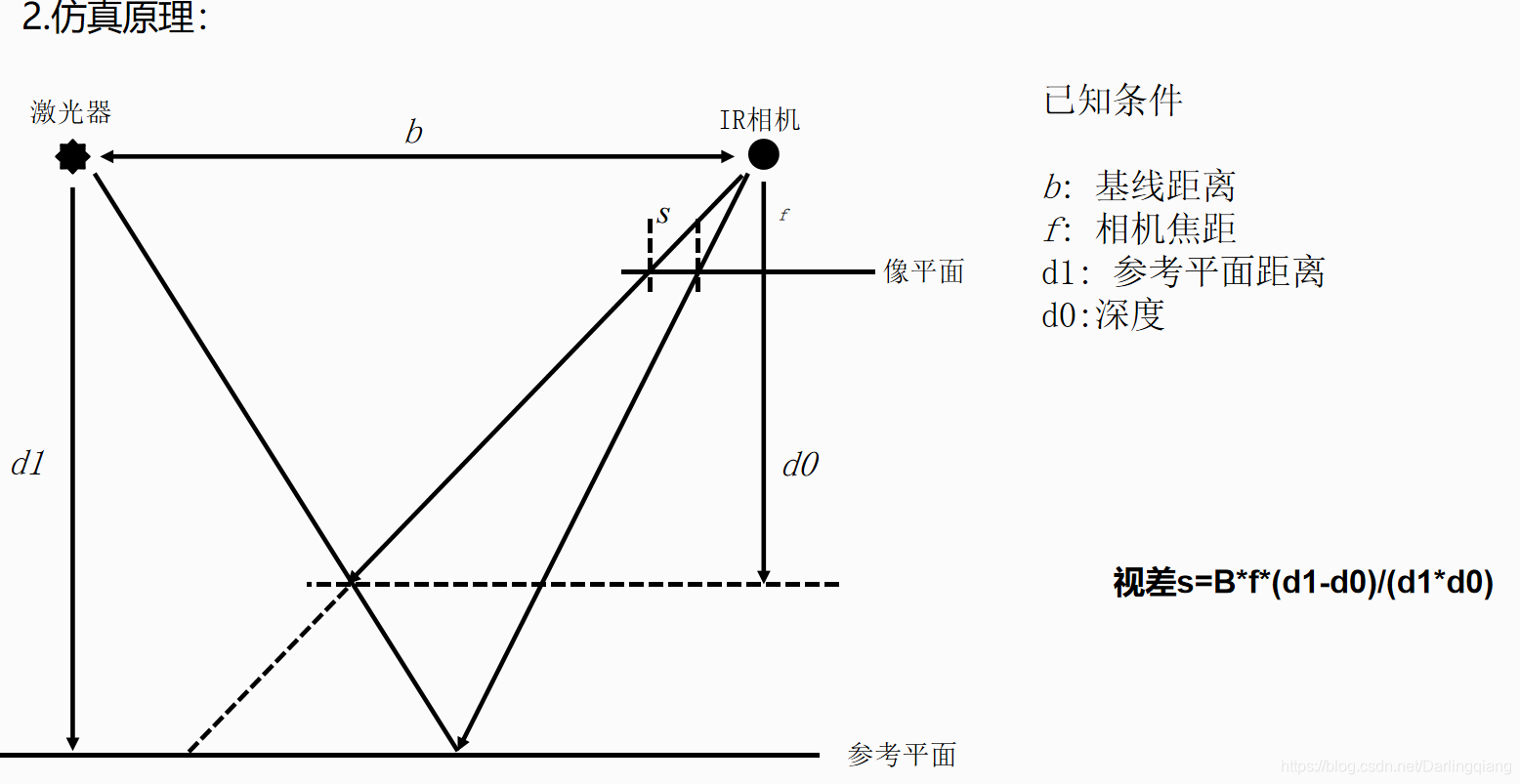
7.投影模型公式 s=B*f*(d1-d0)/(d1*d0);其中其中,B为基线长度,f为焦距,d0为标定距离,d1为当前深度,s为视差。
8.保存数组到txt文件demo.
fileID=fopen([save_path,'scene',num2str(变量),'_obj_info.txt'],'w'); %输出集合数组fmt = '%6f %6f %6f %6f\n'; %%精确到多少位fprintf(fileID,fmt, col2,row2, disparity_x, disparity_y);%保存数组为竖图fclose(fileID);再一次加载:
cur_obj=load([save_path,'scene',num2str(scene_index),'_dis', num2str(distance(dis_index)),'_ref',num2str(d0),'_obj_info.txt']);
9.显示图像,不包含白色边框,保存图片不包含边框。
figure(10000), imshow(obj_image_rot, 'border', 'tight')
image_name=[ 'scene',num2str(d0),'.bmp'];
imwrite(obj_image,[save_path,image_name]);
10.matlab调用exe
[status,result] = system(['C:\bin\RelWithDebInfo\depth_magic_runner.exe "', [save_path,image_name],'" --config "C:\Users\Administrator\Desktop\vescl_after\getconfig"']) ;sttaus返回值为0时,说明程序运行成功,可以通过‘echo’,将输出中间结果打印到屏幕
11.文件更改名称和移动,拷贝等操作。
movefile("debug_output",string(hole_image_name),'f');%改名pause(0.001);movefile(string(hole_image_name),targetPathOri,'f');%移动pause(0.001);由于移动速度比较低,很多的IO读入写入操作,防止程序阻塞可以使用pause等待程序执行完之后再运行其他程序
12.文件检索遍历图片,见https://blog.csdn.net/Darlingqiang/article/details/108286336
13.直方图统计与三维直方图统计
figure(112)
histogram_y = histogram(disparity_y);
title(['y disparity analyze ---- ','y truth mean=',num2str(disparity_y_mean_real_value),',y truth var=',num2str(disparity_y_val_real_value)])
xlabel('the value of disparity y')
ylabel('the histogram of disparity y');
led_y=legend(['y mean=',num2str(disparity_y_mean),' y var=',num2str(disparity_y_var)]);
title(led_y,'speckle center extract ');
saveas(figure(112), [allresult(1).folder, '\disparity_y.bmp'])
% look up biger x bias distribute along x figure(105) histogram_bias_x = histogram2((disparity_diff_matching_x(1:match_num)-disparity_x_mean_real_value),x_ordinate_of_matching_point,...'Normalization','probability','FaceColor','flat'); title('bias x after speckle center extract '); xlabel('x coordinate') ylabel('bias x'); saveas(figure(105), [allresult(1).folder, '\bias_x_after_speckle_center_extract.bmp']);
14.点云处理相关。
读取ply:
data_source=pcread('C:\Users\Administrator\Desktop\vescl\ply\adis800_pc_wave.ply');仿真生成点云参考part two函数:
function [data_target]=scene_to_ply_downsample_function(scene,height,width,distance,multiplier)点云可视化:
figure(1)
point_plane = [z_plane_row,z_plane_col,depth_z_plane];
pc_plane = pointCloud(point_plane);
pcshow(pc_plane);
点云保存:
tic
pcwrite(pc_plane,['adis',num2str(dis),'_pc_plane.ply'],'PLYFormat','ascii');
% pcwrite(pc_plane,['adis',num2str(dis),'_pc_plane.ply'],'PLYFormat','ascii');
toc
part two:函数记录
function [data_target]=scene_to_ply_downsample_function(scene,height,width,distance,multiplier)
输入:对应的场景深度scene1 ,及其对应的宽高,以及当前的仿真距离(也即深度),以及变大或者变小的倍数因子。
function [data_target]=scene_to_ply_downsample_function(scene,height,width,distance,multiplier)% clear;
% close all;
% clc;% dis=300;
% multip =1/2;
% height_low=400;
% width_low=640;
dis=distance;
multip =multiplier;
height_low=height;
width_low=width;
% %***************************** plane  ****************************************************
tx_plane=-height_low:1:height_low-1;
ty_plane=-width_low:1:width_low-1;
[x_plane,y_plane]=meshgrid(tx_plane,ty_plane);%形成格点矩阵
z_plane=0*(10*sin(pi*x_plane/(20))+10*cos(pi*y_plane/(20)));z_plane=imresize(z_plane,multip);[z_plane_row,z_plane_col] = find(z_plane>=-20);
len_z_plane =length(z_plane_row);
depth_z_plane = zeros(len_z_plane,1);
for index_plane = 1:len_z_planez_plane_x =z_plane_row(index_plane,:);z_plane_y =z_plane_col(index_plane,:);  depth_z_plane(index_plane) = z_plane(z_plane_x,z_plane_y)+dis;
end% figure(11)
point_plane = [z_plane_row,z_plane_col,depth_z_plane];
pc_plane = pointCloud(point_plane);
% pcshow(pc_plane);% tic
% pcwrite(pc_plane,['adis',num2str(dis),'_pc_plane.ply'],'PLYFormat','ascii');
% % pcwrite(pc_plane,['adis',num2str(dis),'_pc_plane.ply'],'PLYFormat','ascii');
% toc
% %***************************** step  ****************************************************
% clc;
% close all;
% clear ;
% dis=300;
% multip =1/2;
% height_low=400;
% width_low=640;
z_step(2*height_low,2*width_low) = 0;
for x_step=0:(2*width_low)for y_step=0:(2*height_low)if ((y_step>190)&&(y_step<400)&&(x_step>150)&&(x_step<395))z_step(y_step,x_step) = 4;elseif ((y_step>400)&&(y_step<610)&&(x_step>150)&&(x_step<395))z_step(y_step,x_step) = 1;elseif ((y_step>190)&&(y_step<400)&&(x_step>395)&&(x_step<640))z_step(y_step,x_step) = 3;elseif ((y_step>400)&&(y_step<610)&&(x_step>395)&&(x_step<640))z_step(y_step,x_step) = 2;  elseif ((y_step>190)&&(y_step<400)&&(x_step>640)&&(x_step<885))z_step(y_step,x_step) = 2;  elseif ((y_step>400)&&(y_step<610)&&(x_step>640)&&(x_step<885))z_step(y_step,x_step) = 3; elseif ((y_step>190)&&(y_step<400)&&(x_step>885)&&(x_step<1130))z_step(y_step,x_step) = 1;elseif ((y_step>400)&&(y_step<610)&&(x_step>885)&&(x_step<1130))z_step(y_step,x_step) = 4;    elseif ((y_step<190)&&(y_step>610)&&(x_step<150)&&(x_step>1130))z_step(y_step,x_step) = 1;endend
endz_step=imresize(z_step,multip);
% [rows_step,cols_step]=size(z_step);
[z_step_row,z_step_col] = find(z_step>=-20);
len_z_step =length(z_step_row);
depth_z_step = zeros(len_z_step,1);
for index_step = 1:len_z_stepz_step_x =z_step_row(index_step,:);z_step_y =z_step_col(index_step,:);  depth_z_step(index_step) = z_step(z_step_x,z_step_y)+dis;
end% figure(22)
point_step = [z_step_row,z_step_col,depth_z_step];
pc_step = pointCloud(point_step);
% pcshow(pc_step);
% pcwrite(pc_step,'scene.ply','PLYFormat','ascii')
% tic
% pcwrite(pc_step,['adis',num2str(dis),'_pc_step.ply'],'PLYFormat','ascii');
% toc
% %***************************** wave *********************************************
ty_single=-height_low:1:height_low-1;
tx_single=-width_low:1:width_low-1;
[x_single,~]=meshgrid(tx_single,ty_single);%形成格点矩阵
z_single=10*sin(pi*x_single/(20));%+10*cos(pi*y_wave/(20));
z_single=z_single';
z_single=imresize(z_single,multip);[z_single_row,z_single_col] = find(z_single>=-20);
len_z_single =length(z_single_row);
depth_z_single = zeros(len_z_single,1);
for index_single = 1:len_z_singlez_single_x =z_single_row(index_single,:);z_single_y =z_single_col(index_single,:);  depth_z_single(index_single) = z_single(z_single_x,z_single_y)+ dis;
end% figure(33)
point_wave = [z_single_row,z_single_col,depth_z_single];
pc_wave = pointCloud(point_wave);
% pcshow(pc_wave);% tic
% pcwrite(pc_wave,['adis',num2str(dis),'_pc_wave.ply'],'PLYFormat','ascii');
% toc
% %*****************************  egg  *********************************************
tx_wave=-height_low:1:height_low-1;
ty_wave=-width_low:1:width_low-1;
[x_wave,y_wave]=meshgrid(tx_wave,ty_wave);%形成格点矩阵
z_egg=5*sin(pi*x_wave/(20))+5*cos(pi*y_wave/(20));z_egg=imresize(z_egg,multip);[z_wave_row,z_wave_col] = find(z_egg>=-20);
len_z_wave =length(z_wave_row);
depth_z_wave = zeros(len_z_wave,1);
for index_wave = 1:len_z_wavez_wave_x =z_wave_row(index_wave,:);z_wave_y =z_wave_col(index_wave,:);  depth_z_wave(index_wave) = z_egg(z_wave_x,z_wave_y)+dis;
end% figure(44)
point_plate =[z_wave_row,z_wave_col,depth_z_wave];
pc_egg = pointCloud(point_plate);
% pcshow(pc_egg);if(strcmp(scene,'scene1'))data_target=pc_plane;
elseif(strcmp(scene,'scene2'))data_target=pc_step;
elseif(strcmp(scene,'scene3'))data_target=pc_wave;
elseif(strcmp(scene,'scene4'))data_target=pc_egg;
end
% tic
% pcwrite(pc_egg,['adis',num2str(dis),'_pc_egg.ply'],'PLYFormat','ascii');
% toc
% %***************************** triangular profiler ****************************************************
end
scene_ref_creat_function仿真生成原始散斑
输入设计的vescl pattern输出模拟散斑参考图
function [ref_speckle]=scene_ref_creat_function(center_coordinate)
max_value=800;M=1280;
N=800;
MAX=1023;% 生成一个高斯函数,函数与散斑点的灰度分布具有有较高的一致性,即可以很好的仿真当前的
dia = 1;%散斑直径
sigma = 1;
gausFilter = fspecial('gaussian', [dia,dia], sigma);times=1;%奇数
kernel=imresize(gausFilter,times);%%imresize 使用双三次插值。 B = imresize(A,scale) 返回图像 B,它是将 A 的长宽大小缩放 scale 倍之后的图像。
cx=round(dia*times/2);
cy=round(dia*times/2);
R=floor(dia*times/2);kernel_mask=ones(size(kernel));
for m=1:times*diafor n=1:times*diaif (cx-n)^2+(cy-m)^2>=(R+1)*Rkernel_mask(m,n)=0;endend
endmax_kernel = max(max(kernel));
kernel = kernel.*kernel_mask*(max_value/max_kernel)*0.3;%
IR_speckle=zeros(M*times,N*times);
L=length(center_coordinate);for i=1:Lcenter_x=round(center_coordinate(i,1)*times);center_y=round(center_coordinate(i,2)*times);if(((center_y-R)>0) && ((center_y+R) < M*times) && ((center_x-R)>0) && ((center_x+R) < N*times) ) IR_speckle(center_y-R:center_y+R,center_x-R:center_x+R)=IR_speckle(center_y-R:center_y+R,center_x-R:center_x+R)+ 255;end
endref_speckle=(imresize(IR_speckle,1/times));
ref_speckle(ref_speckle>MAX)=MAX;end
disparity_analyze函数,输入obj_match匹配数组,或者object_info.txt信息,输出匹配点对以及对应的视差
%% 统计六近邻中目标点的视差分布
function [disparity_diff_matching_x,disparity_diff_matching_y,x_ordinate_of_matching_point,y_ordinate_of_matching_point]=disparity_analyze(obj_match)
% obj_info_name = '';
% obj_info_name = dir(fullfile('C:\Users\Administrator\Desktop\vescl_after\result\scene1_dis500_ref400\',obj_info_name,'*object_info*.txt'));% if exist(['C:\Users\Administrator\Desktop\vescl_after\result\scene1_dis500_ref400\' obj_info_name(1).name])
%     obj_match = importdata(['C:\Users\Administrator\Desktop\vescl_after\result\scene1_dis500_ref400\' obj_info_name(1).name]);x_thresholod=0.1;y_thresholod=1;match_list = find(obj_match(:,end)>0);match_num = size(find(obj_match(:,end)>0),1);disparity_diff_x_each_other=zeros(match_num,6);disparity_diff_y_each_other=zeros(match_num,6);disparity_diff_x = zeros(match_num*6,1);% show matching statusdisparity_diff_matching_x=obj_match(match_list(:),end-2);disparity_diff_matching_y=obj_match(match_list(:),end-1);disparity_diff_matching_y_size = size(disparity_diff_matching_y);for i = 1:disparity_diff_matching_y_sizeif(disparity_diff_matching_y(i)>5)disparity_diff_matching_y(i)=0;endendx_ordinate_of_matching_point = obj_match(match_list(:),1);y_ordinate_of_matching_point = obj_match(match_list(:),2);%% disparity_diff_y = zeros(match_num*6,1);disparity_diff_num = 0;for i = 1:match_numobj_num = match_list(i);disp_x = obj_match(obj_num,end-2);disp_y = obj_match(obj_num,end-1);descriptor = obj_match(obj_num,end-8:end-3);desp_list = descriptor(descriptor>0);desp_list = desp_list + ones(size(desp_list));% from one start for j = 1:size(desp_list,2)if obj_match(desp_list(j),end)>0disparity_diff_num = disparity_diff_num + 1;disparity_diff_x(disparity_diff_num) = disp_x - obj_match(desp_list(j),end - 2);if abs(disp_x - obj_match(desp_list(j),end - 2))-x_thresholod >=0 disparity_diff_x_each_other(i,j)=abs(disp_x - obj_match(desp_list(j),end - 2));endif abs(disp_y - obj_match(desp_list(j),end - 1))-y_thresholod >=0 disparity_diff_y_each_other(i,j)=abs(disp_y - obj_match(desp_list(j),end - 1));end% 邻域视差分布问题disparity_diff_y(disparity_diff_num) = disp_y - obj_match(desp_list(j),end - 1);             endend      end%% 统计非零个数cnt_x = zeros(match_num,1);   for i=1:match_numcnt_x(i)= nnz(disparity_diff_x_each_other(i,:)>0);endx_index=find(cnt_x(:));x_size=size(x_index,1);
%  figure
% plot(1:x_size, cnt_x(x_index(:)),'r.')
% title('x disparity diff threshold great 3 distribution ');
% grid on
cnt_y = zeros(match_num,1);   for i=1:match_numcnt_y(i)= nnz(disparity_diff_y_each_other(i,:)>0);endy_index=find(cnt_y(:));y_size=size(y_index,1);%% y 视差 纵坐标 x轴为横坐标
% figure(100)
% plot(1:match_num,disparity_diff_matching_y(1:match_num),'b.')
% title(' y disparity matching result according point num')
% grid on
%
% figure(101)
% plot(y_ordinate_of_matching_point(1:match_num),disparity_diff_matching_y(1:match_num),'b.')
% title(' y disparity matching result along y disparity')
% grid on% figure
% plot(1:disparity_diff_num,disparity_diff_x(1:disparity_diff_num),'r.')
% title('all matching points decriptors x disparity diff ')
% grid on
%
% figure
% plot(1:disparity_diff_num,disparity_diff_y(1:disparity_diff_num),'r.')
% title('all matching points decriptors  y disparity diff ')
% grid on
% figure
% histogram(disparity_diff_x(1:disparity_diff_num),'DisplayStyle','bar')
% title('histogram disparity diff x')
%  saveas(gcf,strcat(root_dir, 'histogram_disparity_diff_x.bmp'));
% figure
% histogram(disparity_diff_y(1:disparity_diff_num),'DisplayStyle','bar')
% title('histogram disparity diff y')   % else
%     disp(['不存在*object_info*.txt'])
% end
end
compute_IoU:求取IOU交并比,可以用于评估重建效果
function [IoU, area] = compute_IoU(region_a, region_b)
%COMPUTE_IOU Is compute the two region overlap area.
%
%   ************************
%   *                      *
%   *      (x_a,y_a)******************
%   *          *           *         *
%   *          *           *         *
%   *          *           *         *
%   *******************(x_b,y_b)     *
%              *                     *
%              *                     *
%              ***********************x_a = max(region_a(1), region_b(1));
y_a = max(region_a(2), region_b(2));
x_b = min(region_a(3), region_b(3));
y_b = min(region_a(4), region_b(4));area_a = (region_a(3) - region_a(1) + 1) * (region_a(4) - region_a(2) + 1);
area_b = (region_b(3) - region_b(1) + 1) * (region_b(4) - region_b(2) + 1);area = max(0, x_b - x_a + 1) * max(0, y_b - y_a + 1);
IoU = area / (area_a + area_b - area);end
scene_creat_function.m 输入宽高,输出场景平面深度图
function [scene1,scene2,scene3,scene4]=scene_creat_function(height,width)
tx_plane=-height/2:1:height/2-1;
ty_plane=-width/2:1:width/2-1;
[x_plane,y_plane]=meshgrid(tx_plane,ty_plane);%形成格点矩阵
z_plane=0*(x_plane+y_plane);
scene1=z_plane;
% %*****************************  SENCE 2 step  ****************************************************
z_step(height,width) = 0;
for x_step=0:widthfor y_step=0:heightif ((y_step>190)&&(y_step<400)&&(x_step>150)&&(x_step<395))z_step(y_step,x_step) = 5;elseif ((y_step>400)&&(y_step<610)&&(x_step>150)&&(x_step<395))z_step(y_step,x_step) = 2;elseif ((y_step>190)&&(y_step<400)&&(x_step>395)&&(x_step<640))z_step(y_step,x_step) = 4;elseif ((y_step>400)&&(y_step<610)&&(x_step>395)&&(x_step<640))z_step(y_step,x_step) = 3;  elseif ((y_step>190)&&(y_step<400)&&(x_step>640)&&(x_step<885))z_step(y_step,x_step) = 3;  elseif ((y_step>400)&&(y_step<610)&&(x_step>640)&&(x_step<885))z_step(y_step,x_step) = 4; elseif ((y_step>190)&&(y_step<400)&&(x_step>885)&&(x_step<1130))z_step(y_step,x_step) = 2;elseif ((y_step>400)&&(y_step<610)&&(x_step>885)&&(x_step<1130))z_step(y_step,x_step) = 5;    elseif ((y_step<190)&&(y_step>610)&&(x_step<150)&&(x_step>1130))z_step(y_step,x_step) = 0;endend
end
scene2=z_step';
% %***************************** SENCE 3 wave *********************************************
ty_single=-height/2:1:height/2-1;
tx_single=-width/2:1:width/2-1;
[x_single,~]=meshgrid(tx_single,ty_single);%形成格点矩阵
z_wave=10*sin(pi*x_single/(20));%+10*cos(pi*y_wave/(20));
scene3=z_wave';
% %***************************** SENCE 4 egg   *********************************************
tx_wave=-height/2:1:height/2-1;
ty_wave=-width/2:1:width/2-1;
[x_wave,y_wave]=meshgrid(tx_wave,ty_wave);%形成格点矩阵
z_egg=5*sin(pi*x_wave/(20))+5*cos(pi*y_wave/(20));
scene4=z_egg;end相关文章:

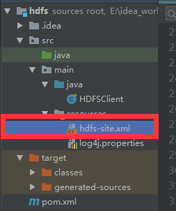
IDEA HDFS客户端准备
在此之前:先进行在IDEA 中为Maven 配置阿里云镜像源 1、将资料包中的压缩包解压到一个没有中文的目录下 2、配置HADOOP_HOME环境变量 3、配置Path环境变量 4、创建一个Maven工程HDFSClientDemo 5、在pom.xml中添加依赖 <dependencies><dependency><g…

12 Java面向对象之多态
JavaSE 基础之十二12 Java面向对象之多态 ① 多态的概念及分类 多态的概念:对象的多种表现形式和能力多态的分类 1. 静态多态:在编译期间,程序就能决定调用哪个方法。方法的重载就表现出了静态多态。 2. 动态多态:在程序运行…
MATLAB【十四】————遍历三层文件夹操作
文件夹遍历 clear; clc; close all;%% crop the im into 256*256 num 0; %% num1 内缩3个像素 num 2 内缩6个像素 load(qualitydata1.mat) load(qualitydata2.mat)[data1_m,data1_n] size(qualitydata1); [data2_m,data2_n] size(qualitydata2);%% read image_name …

LoadRunner监控Linux
有的linux机器上安装rpc后会保存如下: test -z "/usr/local/sbin" || mkdir -p -- . "/usr/local/sbin"/bin/install -c rpc.rstatd /usr/local/sbin/rpc.rstatd make[2]: Nothing to be done for install-data-am. make[2]: Leaving directory…
scala while循环中断
Scala内置控制结构特地去掉了break和continue,是为了更好的适应函数化编程,推荐使用函数式的风格解决break和contine的功能,而不是一个关键字。 如何实现continue的效果 Scala内置控制结构特地也去掉了continue,是为了更好的适应…
05-04-查看补丁更新报告
《系统工程师实战培训》 -05-部署补丁管理服务器 -04-查看补丁更新报告 作者:学 无 止 境QQ交流群:454544014///安装报表工具(在100-Admin01上面安装如下工具,方便查看WSUS更新补丁报告!)Microsoft System CLR Types f…
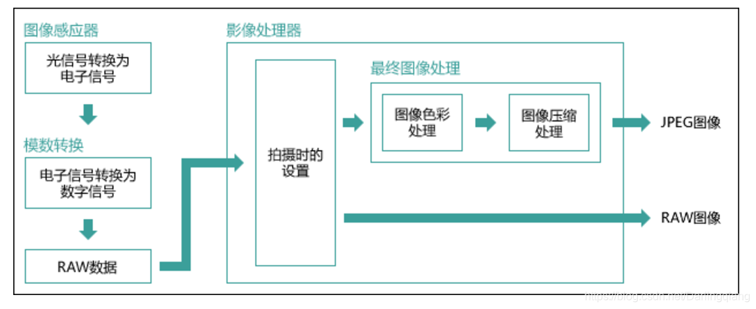
ISP【三】———— raw读取、不同格式图片差异
part zero: 如何处理.raw格式数据,读取和转化 matlab读取raw图 (mark读取图片尺寸和位数均可设置,图片尺寸M,N,图片数据类型8bit,16bit改成uint16) clear; clc; close all; % % rotpath imread(D:\matlab\ncc_ive…

深度学习 - 相关名词概念
2019独角兽企业重金招聘Python工程师标准>>> Neural Network 神经网络 Weights 权重 Bias 偏移 Activation Function 激活函数, 用于调整每个神经的输出, 有如下几个常用的函数种类 ReLU Sigmoid Optimizer 优化器 Adam Input Layer, Hidden Layer, Output Layer 输…
HDFS的API操作
准备工作:IDEA > HDFS客户端准备 目录 文件上传 文件下载 文件夹删除 修改文件名称 查看文件详情 文件和文件夹的判断 完整代码 文件上传 注意conf.set("dfs.replication","2");的位置,位置不一样,设置的副本…
微信小程序-锚点定位+内容滑动控制导航选中
之前两篇文章分别介绍了锚点定位和滑动内容影响导航选中,这里我们就结合起来,实现这两个功能! 思路不再多说,直接上干货! WXML <view class"navigateBox"><view class"title"><ima…
MATLAB【十四】————调用深度库生成exe,批量运行三层文件夹下图片,保存结果
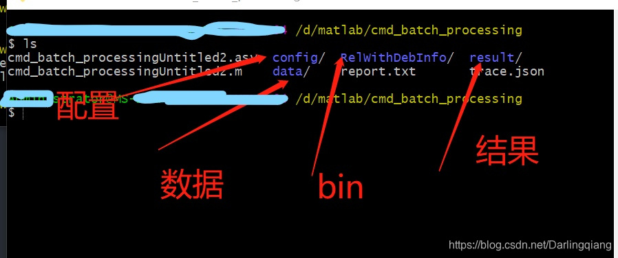
运行路径:D:\matlab\cmd_batch_processing 文件夹架构: clear; clc; close all;%% crop the im into 256*256oriDataPath D:\matlab\cmd_batch_processing\data\; targetPathOri D:\matlab\cmd_batch_processing\result\;report_path D:\matlab\cm…
JDK1.8学习
2019独角兽企业重金招聘Python工程师标准>>> List<OrderGoodsDetail> olist BeanMapper.mapList(list,OrderGoodsDetail.class);List<String> list2 Arrays.asList("123", "45634", "7892", "abch", "s…
HDFS的数据流
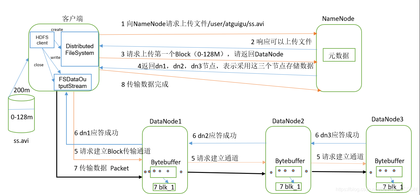
目录 HDFS写数据流程 剖析文件写入 网络拓扑-节点距离计算 机架感知(副本存储节点选择) Hadoop2.7.2 副本节点选择 HDFS读数据流程 HDFS写数据流程 剖析文件写入 1)客户端通过Distributed FileSystem模块向NameNode请求上传文件&#x…
Js----闭包
1、闭包的概念:(我找了很多,看大家的理解) A:闭包是指可以包含自由(未绑定到特定对象)变量的代码块; 这些变量不是在这个代码块内或者任何全局上下文中定义的,而是在定义代码块的环境中定义(局部…
【C++】【四】企业链表
// 企业链表.cpp : 此文件包含 "main" 函数。程序执行将在此处开始并结束。 // 链表改进版 企业常用#include <iostream> #include<stdlib.h>//链表小节点 不包含数据域 typedef struct linknode {struct linknode* next; }linknode; //链表节点 数据指…

GoldenGate的Logdump工具使用简介
Logdump工具是GoldenGate提供的一个用于查询、分析、过滤、查看和保存存储在trail文件或extract文件中的数据的工具。1、启动Logdump工具[oraclerhel6 ~]$ cd /ogg [oraclerhel6 ogg]$ ./logdumpOracle GoldenGate Log File Dump Utility for Oracle Version 12.2.0.1.1 OGGCOR…

scala惰性函数
惰性计算(尽可能延迟表达式求值)是许多函数式编程语言的特性。惰性集合在需要时提供其元素,无需预先计算它们,这带来了一些好处。首先,您可以将耗时的计算推迟到绝对需要的时候。其次,您可以创造无限个集合…
计算机组成原理-第3章-3.1
|--总线:本质上就是一组连线,通路 |--发展过程: 分散连接时代: 运算器为中心 ↓ 存储器为中心 ↓ 中断,DMA的出现修正 ↓ 依旧无法解决效率问题 总线连接时代: 以CPU为核心,双总线:M…
【C++】【三】单向链表
// 单向链表.cpp : 此文件包含 "main" 函数。程序执行将在此处开始并结束。 //#include <iostream> #include<stdlib.h>typedef struct LINKNODE {void* data;struct LINKNODE* next; }linknode;typedef struct LINKLIST {LINKNODE* head;int size; }lin…
gulp相关说明
1.当你按下ctrls 或切换到浏览器,浏览器将会会自动刷新 如果你修改的是html文件将会刷新网页如果你修改的是css或less,这个less文件或css文件将会被重载而不是刷新整个页面(这个特性在写单页面应用时尤为实用)2.模板引入 考虑以下…
IDEA中提示:Warning:java: 源值1.5已过时, 将在未来所有发行版中删除
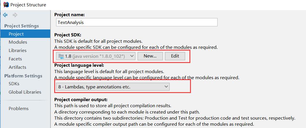
问题描述: 运行Java Web项目时,IDEA中提示:Warning:java: 源值1.5已过时, 将在未来所有发行版中删除解决方法: 1. 打开【File】—【Project Structure】,找到以下两个地方: Project Structure->Proje…
mysql 数据库乱码
mysql 数据库乱码 转载自https://www.cnblogs.com/gne-hwz/p/8748028.html 如有侵权,请联系。 遇到这种情况,现有项目的数据库已经建好,数据表也已经创建完成。 问题来的,数据库不能插入中文,调试时候发现中文数据从发…
【C++】【二】动态数组-Dynamic_linklist
// dynamicArray.cpp : 此文件包含 "main" 函数。程序执行将在此处开始并结束。 // #include <stdlib.h> #include <iostream>typedef struct DYNAMICARRAY {int* paddr;int size;int capacity; }dynamiCarray;dynamiCarray* Init_dynamiCarray() {dynam…
在MySQL和PostgreSQL之外,为什么阿里要研发HybridDB数据库?
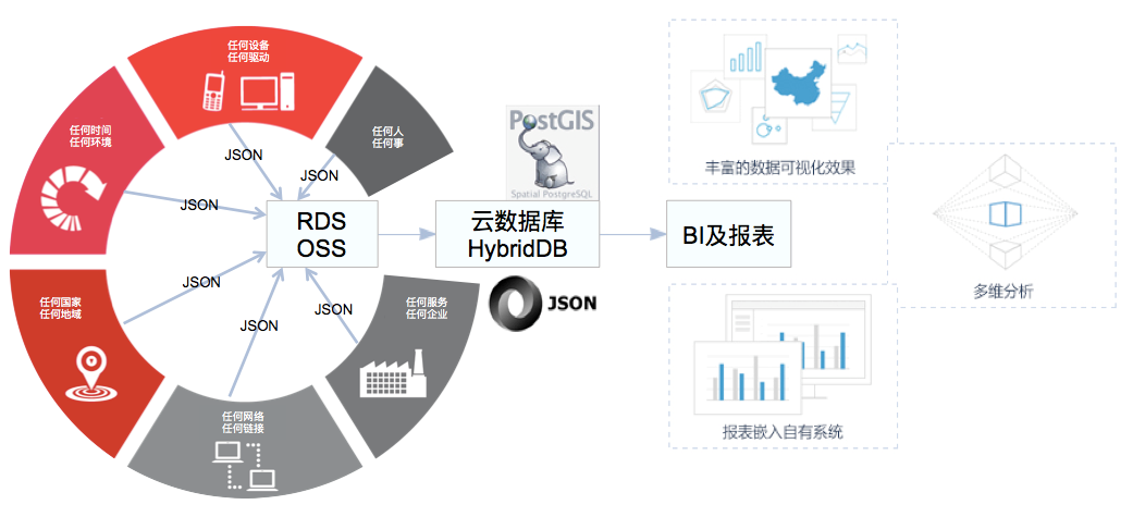
编者按\\在大数据火遍IT界之前,大家对数据信息的挖掘通常聚焦在BI(Business Intelligence)之上。BI具有着明确的分析需求,清晰地知道需要处理哪些信息,并且如何最终获得多维度的SQL类型数据,这种多维度的分…
Linux命令-安装zip和unzip命令
1 [rootiz2zeea05by6vofxzsoxdbz elasticsearch]# unzip elasticsearch-6.2.4.zip 2 -bash: unzip: command not found 如果你如法使用unzip命令解压.zip文件,可能是你没有安装unzip软件,下面是安装方法 命令: yum list | grep zip/unzip …

【C++】【五】循环链表
数据结构:具体的高效有序的管理内存的方法。 链表:数据结构的一种 节点:每一块内存 每一个节点可以是裸指针 也可以是结构体 ,结合企业链表的思路可以将类型强转,完成高效的访问。main.cc // 单向循环链表.cpp …
IntelliJ IDEA 设置项目编码
2019独角兽企业重金招聘Python工程师标准>>> IntelliJ IDEA-> Editor->File Encodings 转载于:https://my.oschina.net/bigxuan/blog/804345
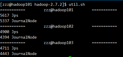
util.sh 脚本
#!/bin/bash for i in zzzhadoop101 zzzhadoop102 zzzhadoop103 doecho " $i "ssh $i /opt/module/jdk1.8.0_144/bin/jps donebin目录是在环境变量里的,所以在哪都可以执行 /home/zzz/bin目录下touch util.sh [zzzhadoop101 bin]$ touch …

bzoj3467: Crash和陶陶的游戏
就一篇题解: BZOJ3467 : Crash和陶陶的游戏 - weixin_34248487的博客 - CSDN博客 1.离线,建出Atrie树;B树的倍增哈希数组,节点按照到根路径字典序排序 2.处理A节点对应前缀对应B中的极长可以匹配的区间。在父亲节点区间内二分即可…